Full Text View

Volume 28, Issue 6 (June 2018)

GSA Today

Article, pp. 4-10 | Abstract | PDF (1.8MB)

Broken Sheets—On the Numbers and Areas of Tectonic Plates

Cover Image

Table of Contents

• Introduction
• Numbers and Areas of Tectonic Plates
• The Broken Sheet Function
• Variation in Plate Size
• Veracity of Plate Subpopulations
• Geographic Clumping of Tectonic Plates
• Discussion
• Implications
• Acknowledgments
• References Cited

 

Search GoogleScholar for

• BH Wilkinson
• BJ McElroy
• CN Dummond

Search GSA Today

 

 

Introduction

The outer brittle layer of the Earth consists of lithospheric plates that move over the relatively weak asthenosphere. Larger-scale aspects of plate movement are the surficial manifestations of mantle convection in the deeper Earth, but local processes of deformation may be only indirectly related to regional stress fields. Because size frequencies from brittle fragmentation might be manifest as self-similar (fractal) power laws (e.g., Davydova and Uvarov, 2013), it is important to know the relationships between lithospheric rheology and degree of fragmentation, as well as the degree to which the breakup of the lithosphere reflects the dynamics of mantle convection versus local interactions along plate boundaries. This is particularly so as models of the evolution of tectonic plates are extended over ever-increasing spans of geologic time (e.g., Domeier and Torsvik, 2014; Matthews et al., 2016; Merdith et al., 2017).

One approach to this question derives from considerations of the numbers and sizes of the tectonic plates. Anderson (2002), for example, noted that fracture patterns tend to self-organize such that mud cracks, frozen ground, basalt columns, and other natural features exhibit similar patterns. He argued that tectonic plates therefore might consist of semi-rigid larger polygons separated by (at times diffuse) boundary zones of deformation surfaced by smaller elements. Bird (2003) presented a global data set interpreted as embodying several fractal subpopulations of plate sizes, each manifest as an approximately linear trend in log area versus log occurrence–frequency space. Sornette and Pisarenko (2003) argued that plate sizes comprise a single continuous power law distribution of size frequency, but with the proviso that a finite Earth surface area imposes an upper limit on larger plate areas. Like Bird (2003), Morra et al. (2013) concluded that plate sizes consist of large and small populations, and that this difference in plate areas persists back in time at least several tens of millions of years. Mallard et al. (2016) employed spherical models of mantle convection to examine the geodynamical processes that drive the tessellation of the Earth’s lithosphere and concurred with Bird (2003) and Morra et al. (2013) that plate areas comprise several distinct populations. Harrison (2016) proposed an additional 107 plates as subdivisions of the 52 plates proposed by Bird (2003); he also interpreted several changes of slope in log-log plots of plate number versus area as reflecting the presence of several size populations.

While the designation of any particular region as a discrete “plate” is somewhat of an evolving enterprise (e.g., Zhang et al., 2017), the actuality of either single (Sornette and Pisarenko, 2003) or multiple (Anderson, 2002; Bird, 2003; Mallard et al., 2016; Harrison, 2016) populations of plate sizes is important to interpreting the manifestation of causative tectonic processes. If sizes of tectonic plates are readily characterized by a single frequency distribution, be it fractal or otherwise, an interpretation of multiple processes operating at distinct length scales is not supported. Conversely, if plate area-frequencies are best described by multimodal distributions, then interpretations linking populations of large plates to processes occurring at convective length scales (e.g., Lenardic et al., 2006) and populations of smaller plates to the generation of lithospheric fragments at the edge of plate boundaries are entirely reasonable.

Numbers and Areas of Tectonic Plates

Detailed data on major tectonic boundaries and areas of enclosed plates are summarized by Bird (2003), who presented the characteristics and locations of 6,048 points that serve to define 229 boundary segments delineating 52 lithospheric plates. The relationship between plate area and frequency of occurrence is most conveniently represented as a cumulative frequency distribution in which plate area is plotted relative to size exceedance—the number of plates equal to or larger than any size in question; the Y-intercept defines the total number (e.g., 52) of data values (Fig. 1).

Figure 1
Areas of tectonic plates relative to exceedance, the number of plate areas equal to or greater than the x-axis values. (A) Plate areas from Bird (2003). (B) Areas from Gurnis et al. (2012). Division into three apparent subpopulations in (A) (n = 52) and two subpopulations in (B) (n = 20) is based on seemingly linear trends (straight red lines). Light blue lines in (A) are 500 sets of plate areas (n = 52) resampled from a stable model time series wherein two random plates are annealed and another two randomly divided over thousands of iterations (see text). Heavy blue line in (A) is the average area of many realizations of such annealed and broken plates. Light brown lines in (B) are 500 sets of plate areas (n = 20) resampled from the broken sheet density function. Heavy brown line in (B) is the ideal broken sheet size frequency distributions predicated by the number of designated plates (20) and the total area of the sphere on which they exist (4 π steradians; ~510 × 10⁶ km²). White lines in (A) and (B) are the two series whose areas, by chance, are closest to observed sizes. Since there is no inherent division of sizes in these models, any subdivision based on the perception of differing slopes for straight-line segments is spurious.

The Broken Sheet Function

The general curvilinear form of log-log plate area frequency distributions is similar to size-frequency distributions for some other area mosaics that include regions of like sediment (lithotopes) across depositional surfaces (Wilkinson and Drummond, 2004), regions on global geologic maps (Wilkinson et al., 2009), sizes of geopolitical subdivisions (McElroy et al., 2005), and taxonomic divisions of organismal morphospace (Wilkinson, 2011). Size-frequency distributions for these tessellations reflect the partitioning of the total area into mosaics of sub-elements wherein locations of boundaries, and therefore the sizes of these elements, are statistically independent.

Conceptually, if the sizes of sub-elements are represented by linear distances across them rather than areas, the distribution of distances between boundaries is the same as that arising from the classic one-dimensional “broken stick” model of random linear subdivision proposed by MacArthur (1957), who suggested that ecological niches within a resource pool could be broken up like a stick, with each piece of the stick representing a niche occupied in the community. This one-dimensional style of division comprises an exponential distribution of separation magnitudes, the same as that arising from differences between a series of ordered random numbers. In the two-dimensional manifestation of random division, a scenario that herein we refer to as the “broken sheet” model, area-frequency distributions are those that would result when linear distances between each boundary are exponentially distributed. The broken sheet distribution (e.g., Fig. 1) is the form that results when sizes of randomly partitioned sub-elements are plotted as areas, rather than distances. The surface of the Earth can therefore be described as being subdivided into tectonic plates such that plate sizes, as measured by the linear distances across them, are exponentially distributed and, hence, like the broken stick, are consistent with random subdivision.

In the broken sheet size-frequency distribution, size exceedance (E, the number of plates with areas greater than or equal to some value) of any entity with some area (A) is defined by the relation in Equation (1),

E = n e^(−Ap2)0.5,      (1)

where n is the total number of entities, p is the incidence of boundary occurrence—the probability of crossing some boundary per unit length of transect, itself expressed as Equation (2),

p = 0.5 nπ/A^0.5,      (2)

and A is the total surface or “sheet” area being divided (for Earth, ~510 × 10⁶ km²).

Comparisons to the 52 plate areas from Bird (2003) and the 20 plate areas from Gurnis et al. (2012) yield R² values of 0.87 and 0.93, respectively (Fig. 1); values of p, which correspond to the probability of crossing a plate boundary, are ~0.045% and 0.025% per kilometer, respectively.

Variation in Plate Size

If a broken sheet distribution describes the sizes of lithospheric plates more effectively than the multi-fractal (e.g., Bird, 2003; Morra et al., 2013; Harrison, 2016) systems proposed earlier, then this system should also: (1) largely account for differences between these theoretical size frequency distributions and those observed among measured plate areas; and (2) yield results that are in agreement with the apparent grouping of plate areas into the several subpopulations based on apparent linear trends in log-log plot of area versus exceedance (e.g., Fig. 1). With respect to differences between theoretical and observed plate areas, it seems apparent that increases in the size of any particular plate might occur fairly continuously through marginal accretion during seafloor spreading or more abruptly during the development of tectonic sutures at convergent margins, and that decreases might occur continually during subduction, or relatively episodically during the development of rifted or transform boundaries. Modern plate size frequencies are a snapshot of the time-integrated geologic histories of the growth and decline in the numbers and sizes of all constituents of the global plate population (e.g., Morra et al., 2013).

A straightforward model of such processes might simply presume that the observed lithospheric plate area frequency distribution is a natural consequence of both the random division and random annealing of members of some initial population of plate areas. We effect such a simulation with a population of n = 52 plates (e.g., Bird, 2003), each with an initial area of 9.8 × 10⁶ km² (A = 510 × 10⁶ km²). From this group, one pair is selected at random and annealed into a single composite; another element is then selected and randomly divided. Because some minimum area should serve to separate lithospheric “plates” and smaller structural elements, we assume a minimum area of 4,000 km², about half the size of the smallest (Manus, 8,117 km²) plate in the Bird (2003) database. Moreover, owing to constraints imposed by length scales of mantle convection (e.g., Lenardic et al., 2006), we assume a maximum plate area of 200 × 10⁶ km², about twice the area of the largest (Pacific, 104 × 10⁶ km²) plate. Given these two constraints, repeated annealing and division of members of the population rapidly results in model size frequencies that are both stable with respect to numbers of iterations and indistinguishable from the observed frequency distribution of modern plate areas (Fig. 1A). The range of permissible area frequencies afforded by this simple model of repeated random annealing and fragmentation completely overlaps the observed sizes of Bird’s (2003) 52 plates.

Veracity of Plate Subpopulations

A single “broken sheet” hypothesis for the generation of a continuum of plate sizes must also account for the widely held perception that plate areas somehow comprise two or more subpopulations, each scaled to some distinct tectonic processes. We suggest that what appear to be “population-specific” segments in log-size versus log-exceedance plots (Fig. 1) are no more than coincidental trends in a sparsely sampled continuum of plate areas. Two issues are relevant to the veracity of dividing and interpreting curvilinear log-log data arrays on the basis of apparent straight line segmentation. First, any model that includes a greater number of subdivisions and a greater number of parameters (each line segment being described by some slope and intercept) will certainly result in better agreement with data than one with fewer parameters (only the number of plates and total area comprise the broken sheet representation). However, benefits from increases in goodness-of-fit are balanced by costs in model complexity (e.g., Akaike, 1974), and greater numbers of model parameters run counter to the heuristic perception that simpler is better. Furthermore, any array representing some sparsely sampled curvilinear distribution will unavoidably exhibit runs of apparent linearity (e.g., Fig. 2). Are the several subpopulations of plate areas suggested by Bird (2003), Morra et al. (2013), Harrison (2016), and Mallard et al. (2016) statistically distinct from apparently linear runs manifest in the sparse sampling of a broken sheet?

Figure 2
Correlations and slopes of apparent linear trends in measured and model plate area frequencies. (A) Plate areas from Gurnis et al. (2012) exhibiting an apparent inflection in slope at log area ~7.7 (~50 × 10⁶ km²); slope difference is 2.11. (B) Two model area frequency distributions, each comprising 20 randomly delimited plate areas with a total of 510 × 10⁶ km²; red and blue lines represent the two best-fit log-linear regressions that account for the largest amount of plate size variance. (C) Frequency distribution of R² values of 1,000 models of 20 randomly delimited plate areas (light yellow bars) compared to R2 values of smaller (red bar, red line in [A]) and larger (blue bar, blue line in [A]) “populations” in the Gurnis et al. (2012) data. (D) Frequency distribution of apparent differences in slopes of “smaller” (e.g., red lines in [B]) and “larger” (e.g., blue lines in [B]) plate areas among 1,000 models of 20 randomly delimited plate areas (tan bars) compared to that defined by smaller (red line in [A]) and larger (blue line in [A]) plate “populations” in the Gurnis et al. (2012) data (brown bar). Note that area-exceedance correlations of “small” and “large” plate areas in the observed data as well as differences in these slopes all fall well within the range of values expected for the sparse sampling of a continuous broken sheet distribution of plate areas.

In order to address that question, we consider the tabulation of 20 plate areas from Gurnis et al. (2012) used by Morra et al. (2013) to define two subpopulations of plate sizes (Figs. 1B and 2A). As noted, these plate sizes are closely approximated by areas in which diameters are exponentially distributed—the broken sheet function (Fig. 1B). If we randomly draw a sample of 20 areas from such a theoretical population, by chance the resultant array will exhibit some number of apparent linear runs in log plate area versus log exceedance space (Fig. 2B). In order to quantify the degree of spurious linearity apparent in such randomly sampled populations, we repeatedly calculate the slopes and correlation coefficients for the two linear trends that most closely match the sample areas in such a model array, determine the sample (plate) number and area where the intersection between these two linears occurs, and calculate the differences in their slopes. Based on this exercise, it becomes apparent that the R² values of all spurious linear arrays (Fig. 2C), as well as the differences between their slopes (Fig. 2D), comprise populations that completely overlap similar parameters derived from the Gurnis et al. (2012) data. Because we cannot reject the null hypothesis that all of these areas were drawn from the same size-frequency distribution, any proposition that they somehow exemplify several distinct subpopulations of plate areas becomes untenable. Proposed linear runs of plate areas are entirely consistent with the sparse sampling of a broken sheet.

Geographic Clumping of Tectonic Plates

Given that a broken sheet model of plate fragmentation, wherein geographic locations of plate boundaries are randomly distributed across the Earth’s surface, is in good agreement with observed areas of plates (Fig. 1), we might then ask if the Earth’s plates also exhibit random geographic dispersal. If the distribution of plate boundaries was laterally homogeneous, then it follows that the areas of those plates should be spatially homogeneous as well; that is, the numbers of plates within some distance of the centroid of any other plate might exhibit a unimodal distribution. Conversely, if plates were geographically associated by size, then numbers of neighbors within some distance of any plate center might exhibit some sort of multimodal frequency distribution, with smaller distances separating smaller plate centroids, and larger distances separating larger. Among the Bird (2003) data, the closest pair of centroids is that of the North Bismarck and Manus plates off Papua New Guinea (235 km); no plates have any neighbors within a smaller distance. Conversely, the most widely separated centers are those of the South American and Philippine Sea plates (19,412 km); at that (or any greater) distance, all centroids have 51 neighbors. Taking 5,000 km as a working distance, the frequency of so-defined neighbors for any one of the Bird (2003) plates ranges from 1 to 23 (Fig. 3). Moreover, Monte Carlo simulations show that the number of neighbors within 5,000 km of randomly distributed centroids in fact does comprise a Gaussian distribution with a mode of ~8 neighbors, the modal number expected for the centroids of 52 plates haphazardly dispersed across ~510 × 10⁶ km² of the Earth’s surface (Fig. 3). Because several plates exhibit numbers of neighbors that fall well above 95% confidence limits for randomly placed centroids, we can reject the null hypothesis that the distribution of plate sizes is truly random. Those observed plates with 17 or more neighbors within 5,000 km (Fig. 3) are located exclusively in the southwestern Pacific; no other part of the Earth exhibits a statistically significant concentration of tectonic plates.

Figure 3
Number of neighbor plate centers within 5,000 km of plate centroids (bars) and Monte Carlo simulation of numbers of neighbors apparent among 500 model sets of randomly distributed plate centers (yellow envelope). Names of several larger plates and those with fewest (African) and most (north Bismarck) neighbors are above appropriate bars. Note that 16 plates have 17 or more neighbors (darker red bars), a density that reflects a spatial association of smaller plates; all of these occur in the southwestern Pacific.

Discussion

Numbers and Sizes of Tectonic Plates

In general, the numbers and areas of modern tectonic plates are closely replicated by the distributions expected when locations of boundaries are largely independent; to a first approximation, the Earth’s lithospheric surface is randomly subdivided. That several smaller plates exhibit geographic association also suggests that actual fragmentation is more accurately characterized as a spatially heterogeneous Poisson process; the probability of crossing some plate boundary varies with geographic position, being higher across the southwestern Pacific.

Understanding the reasons for differing numbers and sizes of tectonic plates is important from a number of perspectives. As noted, difference in plate areas might implicate different processes in their evolution, with larger plates being carried and transported by mantle convection and smaller ones undergoing greater amounts of brittle deformation along regions of convective convergence. The greatest clustering of plates is around the equatorial North Bismarck plate off Papua New Guinea (23 neighbors within 5,000 km). Association of smaller plates in the southwestern Pacific could reflect a greater importance of such processes of plate fracture, particularly when overriding plates are oceanic lithosphere, in ways that are not associated with convergence when the overriding plate is continental lithosphere, as is found along the eastern Pacific. However, fragmentation alone is a uni­directional process that serves to abruptly decrease plate sizes and somewhat obviates considerations of size changes that might arise through subduction, spreading, or suturing.

Although identification of “populations” of large and small plates defined by apparent linear runs in log size versus log exceedance space may indeed be spurious, this does not preclude an interpretation that plate-center convection and plate-margin tectonism have differentially influenced plate size histories. There is much support for the premise that the mechanisms of plate formation and destruction might exhibit a degree of variation along a theoretical length scale. At a longer scale, it is generally accepted, for example, that larger plates bearing continental crust tend to aggregate over cold downwellings, leading to overheating of the mantle, which in turn gives rise to the tensional fragmentation of continents (e.g., Gurnis, 1988). Conversely, at a shorter scale, subduction zones may tend to produce smaller plates (e.g., Mallard et al., 2016), particularly when subduction-related back-arc volcanism develops into oceanic spreading centers (e.g., Bird, 2003); microplates may also be produced along seafloor spreading centers when propagating rifts pass by each other (e.g., Hey et al., 1985). Other processes of plate generation and destruction are less sensitive to length scale; plates of any size can be amalgamated during continental collision and/or destroyed by subduction.

That plate areas are in general agreement with the premise that the Earth’s lithosphere is randomly fragmented, yet there is geographic association of larger and smaller plates, merely enforces the supposition that those factors responsible for the generation of differing plate numbers, sizes, and locations, both in time and in space, must reflect a concatenation of many complex processes, but that these processes also operate with differing geographic and/or temporal intensity across the Earth’s surface.

Implications

As a first approximation, the Earth’s lithosphere generally comprises a randomly broken sheet wherein the occurrences of plate boundaries are spatially independent but somewhat geographically clustered across the southwestern Pacific. This suggests that the processes of spreading, suturing, fragmentation, and subduction, which ultimately result in differing plate areas as well as contiguous areas of granitic crust (i.e., continents), are irreconcilably complex while also exhibiting some degree of spatial and temporal heterogeneity across the Earth’s surface. The Earth’s evolving tectonic state, particularly with respect to continental fragmentation, serves to influence ocean currents, atmospheric composition, and circulation, as well as balances of incoming and outgoing radiation; the location of elevated terrain suitable for the development of glacial ice forces climate change, which in turn serves to modulate rates of geochemical cycling through atmospheric and oceanic reservoirs (e.g., DeConto, 2009). Wilson cycle–scale changes in degree of continental amalgamation and dispersal have been invoked as causal drivers for a wide variety of large-scale processes ranging from changes in continental freeboard (e.g., Whitehead and Clift, 2009) to climatic and biogeochemical cycling (e.g., Nance and Murphy, 2013) to global marine animal diversity (e.g., Zaffos et al., 2017). As such, the broken sheet model serves as a first-order metric for the quantification of changes in extents of continental aggregation over geologic time.

From a practical point of view, the broken sheet function or a derivative thereof can serve as a useful metric in describing size frequencies in many systems where entity size is measured as some area, and where log size versus log exceedance (cumulative count) comprise curvilinear arrays in log-log space, as is the case with respect to some compilations of calderas (e.g., Geyer and Martí, 2012), impact craters (e.g., Hergarten and Kenkmann, 2015), and earthquake magnitudes (e.g., Kagan, 2002). With respect to lithospheric plates, Mallard et al. (2016) have recently noted that specifics concerning how plate sizes relate both to properties of the lithosphere and processes of underlying mantle convection are poorly understood. In order to address these questions, they employ three-dimensional spherical models of mantle convection that combine pseudo-plasticity and variations in viscosity in order to generate plate-like behavior (Fig. 4A). Pseudo-plasticity is realized through a yield stress that characterizes the plastic limit at which concentrated strain produces plate boundaries. Their models produce plate size–frequency distributions that serve to more intimately relate styles of lithosphere fragmentation to processes of mantle convection. Perhaps not surprisingly, lower values of yield stress correspond to greater degrees of fragmentation. But this relation is more readily quantified when transition probabilities are determined for degrees of fragmentation at differing yield stresses. Specifically, transition probability (Tp) decreases (lithosphere fragmentation increases) with increasing yield stress (Ys) as: Tp = 0.108 Ys^−1.14; R² = 0.95 (Fig. 4). From a utilitarian perspective, the broken sheet function therefore appears to effectively capture degrees of lithospheric tessellation under differing rheological conditions and therefore affords a potentially useful metric for describing the evolution of crustal deformation over the entire span of Earth’s geologic history.

Figure 4
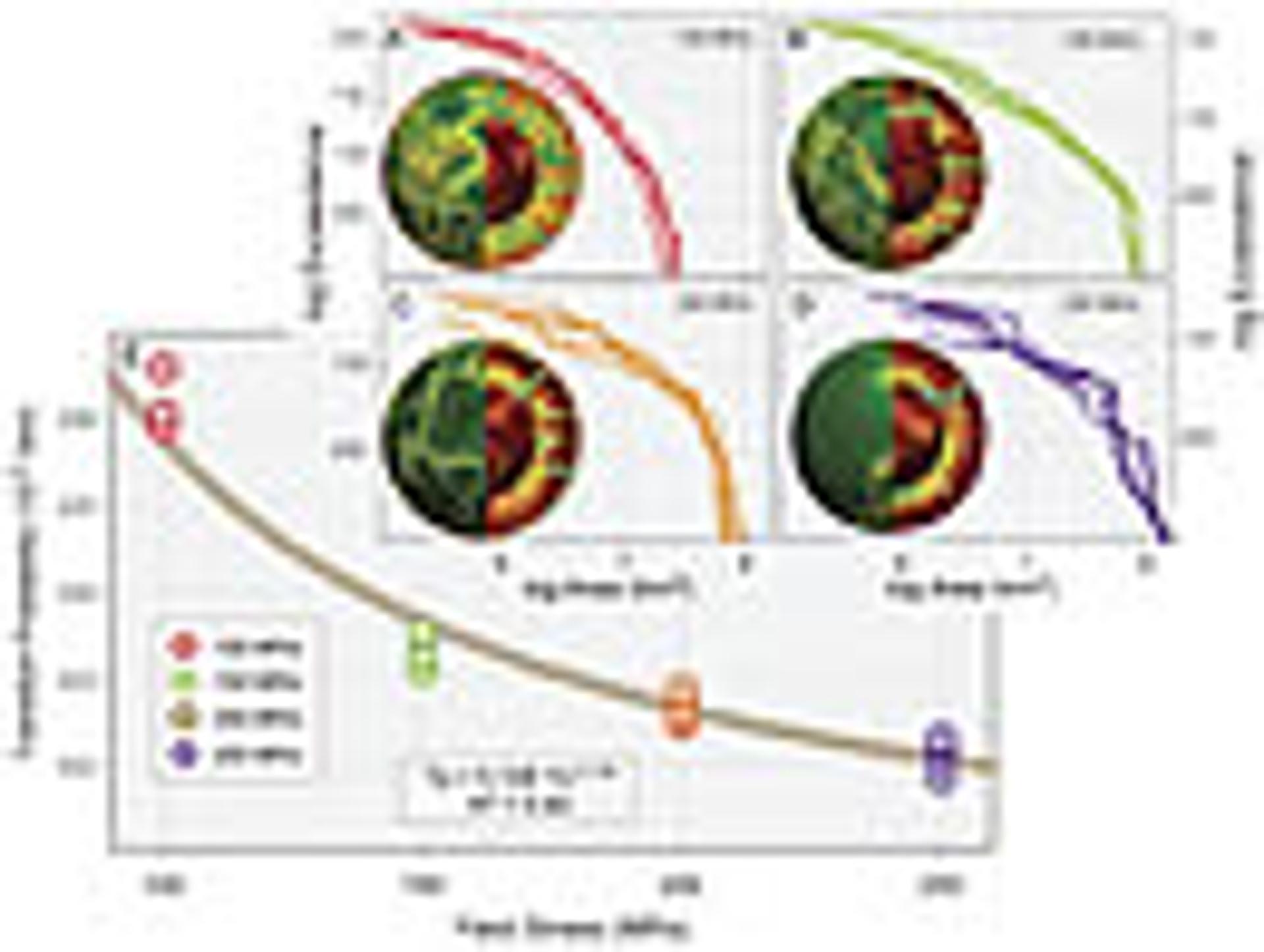
(A–D) Convection in 3D spherical models of mantle convection (inset Earth models) and the logarithm of plate size versus log exceedance (cumulative count) (colored lines) for yield stresses of 100, 150, 200, and 250 MPa from Mallard et al. (2016). (E) Transition probabilities for broken sheets calculated for the 18 arrays of plate area and number (colored lines in [A–D]). Relations between model yield stresses and transitions probabilities defined an approximate power law relation between stress at model plate boundaries and degree of plate fragmentation.

From a more philosophical point of view, understanding the nature of size frequencies of tectonic plates, continents, and other entities is perhaps of more than just academic interest. The study of many geologic features commonly generates quite dissimilar interpretations, and these disagreements often arise from inherently different perceptions of our world. On the one hand, a deterministic view links the origins of observed phenomena to unique and discernable causes in an explainable way, while on the other, a more stochastic perspective argues that the concatenation of multiple intricate geologic processes gives rise to a large degree of randomness and generally unresolvable levels of complexity in the natural world. Where one falls on this spectrum bears directly on how one interprets the numbers and sizes of tectonic plates and the reality of proposed linkages between a rather deterministic understanding of regional motions of the asthenosphere and those more complex and decidedly less predictable processes of local deformation.

Acknowledgments

Details of this analysis profited from discussions with many individuals in the Department of Earth Sciences at Syracuse University; input from Joe Kula, Jim Metcalf, and Scott Miller was particularly valuable. We thank Jerry Dickens for encouragement to write the paper and Claire Mallard for sharing data on numbers and areas of plates from her three-dimensional spherical models of mantle convection. Peter Bird, Christopher Harrison, Linda Ivany, and Greg Hoke read drafts of the manuscript and offered many helpful comments and suggestions.

References Cited

1. Akaike, H., 1974, A new look at the statistical model identification: IEEE Transactions on Automatic Control, v. 19, p. 716–723, https://doi.org/10.1109/TAC.1974.1100705.
2. Anderson, D.L., 2002, How many plates?: Geology, v. 30, p. 411–414, https://doi.org/10.1130/0091-7613(2002)030<0411:HMP>2.0.CO;2.
3. Bird, P., 2003, An updated digital model of plate boundaries: Geochemistry Geophysics Geosystems, v. 4, p. 1–52, https://doi.org/10.1029/2001GC000252.
4. Davydova, M., and Uvarov, S., 2013, Fractal statistics of brittle fragmentation: Frattura ed Integrità Strutturale, v. 24, p. 60–68, https://doi.org/10.3221/IGF-ESIS.24.05.
5. DeConto, R.M., 2009, Plate tectonics and climate change, in Gornitz, V., ed., Encyclopedia of Paleoclimatology and Ancient Environments: Amsterdam, Springer-Verlag, p. 784–798, https://doi.org/10.1007/978-1-4020-4411-3_188.
6. Domeier, M., and Torsvik, T.H., 2014, Plate tectonics in the late Paleozoic: Geoscience Frontiers, v. 5, p. 303–350, https://doi.org/10.1016/j.gsf.2014.01.002.
7. Geyer, A., and Martí, J., 2012, Applying Benford’s law to volcanology: Geology, v. 40, p. 327–330, https://doi.org/10.1130/G32787.1.
8. Gurnis, M., 1988, Large-scale mantle convection and the aggregation and dispersal of supercontinents: Nature, v. 332, p. 695–699, https://doi.org/10.1038/332695a0.
9. Gurnis, M., Turner, M., Zahirovic, S., DiCaprio, L., Spasojevic, S., Müller, R.D., Boyden, J., Seton, M., Manea, V.C., and Bower, D.J., 2012, Plate tectonic reconstructions with continuously closing plates: Computers and Geosciences, v. 38, p. 35–42, https://doi.org/10.1016/j.cageo.2011.04.014.
10. Harrison, C.A.G., 2016, The present-day number of tectonic plates: Earth, Planets, and Space, v. 68, no. 37, p. 3–14, https://doi.org/10.1186/s40623-016-0400-x.
11. Hergarten, S., and Kenkmann, T., 2015, The number of impact craters on Earth—Any room for further discoveries?: Earth and Planetary Science Letters, v. 425, p. 187–192, https://doi.org/10.1016/j.epsl.2015.06.009.
12. Hey, R.N., Naar, D.F., Kleinrock, M.C., Phipps Morgan, J.W., Morales, E., and Schilling, J.G., 1985, Microplate tectonics along a superfast seafloor spreading system near Easter Island: Nature, v. 317, p. 320–325, https://doi.org/10.1038/317320a0.
13. Kagan, Y.Y., 2002, Seismic moment distribution revisited: I. Statistical results: Geophysical Journal International, v. 148, p. 520–541, https://doi.org/10.1046/j.1365-246x.2002.01594.x.
14. Lenardic, A., Richards, M.A., and Busse, F.H., 2006, Depth-dependent rheology and the horizontal length scale of mantle convection: Journal of Geophysical Research, v. 111, B07404, https://doi.org/10.1029/2005JB003639.
15. MacArthur, R.H., 1957, On the relative abundances of birds: Proceedings of the National Academy of Sciences of the United States of America, v. 43, p. 293–295, https://doi.org/10.1073/pnas.43.3.293.
16. Mallard, C., Coltice, N., Seton, M., Müller, D., and Tackley, P.J., 2016, Subduction controls the distribution and fragmentation of Earth’s tectonic plates: Nature, v. 535, p. 140–143, https://doi.org/10.1038/nature17992.
17. Matthews, K.J., Maloney, K.T., Zahirovic, S., Williams, S.E., Seton, M., and Müller, R.D., 2016, Global plate boundary evolution and kinematics since the late Paleozoic: Global and Planetary Change, v. 146, p. 226–250, https://doi.org/10.1016/j.gloplacha.2016.10.002.
18. McElroy, B.J., Wilkinson, B.H., and Rothman, E.D., 2005, Tectonic and topographic framework of political division: Mathematical Geology, v. 37, p. 197–206, https://doi.org/10.1007/s11004-005-1309-2.
19. Merdith, A.S., Williams, S.E., Müller, R.D., and Collins, A.S., 2017, Kinematic constraints on the Rodinia to Gondwana transition: Precambrian Research, v. 299, p. 132–150, https://doi.org/10.1016/j.precamres.2017.07.013.
20. Morra, G., Seton, M., Quevedo, L., and Müller, D., 2013, Organization of the tectonic plates in the last 200 Myr: Earth and Planetary Science Letters, v. 373, p. 93–101, https://doi.org/10.1016/j.epsl.2013.04.020.
21. Nance, R.D., and Murphy, J.B., 2013, Origins of the supercontinent cycle: Geoscience Frontiers, v. 4, p. 439–448, https://doi.org/10.1016/j.gsf.2012.12.007.
22. Sornette, D., and Pisarenko, V., 2003, Fractal plate tectonics: Geophysical Research Letters, v. 30, p. 5-1–5-4.
23. Whitehead, J.A., and Clift, P.D., 2009, Continent elevation, mountains, and erosion: Freeboard implications: Journal of Geophysical Research, v. 114, p. 1–12, https://doi.org/10.1029/2008JB006176.
24. Wilkinson, B.H., 2011, On taxonomic membership: Paleobiology, v. 37, p. 519–536, https://doi.org/10.1666/10024.1.
25. Wilkinson, B.H., and Drummond, C.N., 2004, Facies mosaics across the Persian Gulf and around Antigua—Stochastic and deterministic products of shallow-water sediment accumulation: Journal of Sedimentary Research, v. 74, p. 513–526, https://doi.org/10.1306/123103740513.
26. Wilkinson, B.H., McElroy, B.J., Kesler, S.E., Peters, S.E., and Rothman, E.D., 2009, Global geologic maps are tectonic speedometers—Rates of rock cycling from area-age frequencies: Geological Society of America Bulletin, v. 121, p. 760–779, https://doi.org/10.1130/B26457.1.
27. Zaffos, A., Finnegan, S., and Peters, S.E., 2017, Plate tectonic regulation of global marine animal diversity: Proceedings of the National Academy of Sciences of the United States of America, v. 114, p. 5653–5658, https://doi.org/10.1073/pnas.1702297114.
28. Zhang, T., Gordon, R.G., Mishra, J.K., and Wang, C., 2017, The Malpelo Plate Hypothesis and implications for nonclosure of the Cocos-Nazca-Pacific plate motion circuit: Geophysical Research Letters, v. 44, p. 8213–8218, https://doi.org/10.1002/2017GL073704.

top