In this article
Authors
Bilal U. Haq
Smithsonian Institution, Washington, D.C., USA, and Sorbonne University, Paris, France
Abstract
Documentation of eustatic variations for the Triassic is limited by the paucity of the preserved marine stratigraphic record, which is confined mostly to the low and middle paleolatitudes of the Tethys Ocean. A revised sea-level curve based on reevaluation of global stratigraphic data shows a clear trend of low seastands for an extended period that spans almost 80 m.y., from the latest Permian to the earliest Jurassic. In the Early and Middle Triassic, the long-term sea levels were similar to or 10–20 m higher than the present-day mean sea level (pdmsl). This trend was reversed in the late Ladinian, marked by a steady rise and culminating in peak sea levels of the Triassic (~50 m above pdmsl) in the late Carnian. The trend reverses again with a decline in the late Norian and the base level remaining close to the pdmsl, and then dipping further in the mid-Rhaetian to ~50 m below pdmsl into the latest Triassic and earliest Jurassic. Superimposed upon this long-term trend is the record of 22 widespread third-order sequence boundaries that have been identified, indicating sea-level falls of mostly minor (<25 m) to medium (25–75 m) amplitude. Only six of these falls are considered major, exceeding the amplitude of 75 m. The long interval of Triassic oceanic withdrawal is likely to have led to general scarcity of preserved marine record and large stratigraphic lacunae. Lacking evidence of continental ice sheets in the Triassic, glacio-eustasy as the driving mechanism for the third-order cyclicity can be ruled out. And even though transfer of water to and from land aquifers to the ocean as a potential cause is plausible for minor (a few tens of meters) sea-level falls, the process seems counter-intuitive for third-order events for much of the Triassic. Triassic paleoenvironmental scenarios demonstrate a close link between eustasy, climates, and biodiversity.
Manuscript received 17 July 2018. Revised manuscript received 22 Sept. 2018. Manuscript accepted 28 Sept. 2018. Posted 10 Oct. 2018.
© The Geological Society of America, 2018. CC-BY-NC.
Introduction
The Triassic Period encompasses 50.5 m.y., spanning an interval from 251.9 to 201.4 Ma (Ogg et al., 2016). By this time, the megacontinent of Pangaea had already assembled, surrounded by the Panthalassa Ocean that covered >70% of Earth’s surface, and by the mid-Triassic the Pangaean landmass was almost evenly distributed in the two hemispheres around the paleo-equator (see Fig. S1 in the GSA Data Repository1). The interval from latest Permian through the earliest Jurassic, a time span of nearly 80 m.y., represents the longest spell of low seastands of the Phanerozoic. The Triassic is also bracketed by two major biotic extinctions near the Permian-Triassic (P-T) and Triassic-Jurassic boundaries, the one at P-T boundary being the most severe biotic turnover of the Phanerozoic (Raup and Sepkowski, 1982; Hallam and Wignall, 1997; McElwain et al., 1999). The Late Triassic experienced the beginning of the lithospheric swell, ushering the breakup of Pangaea and its eventual split into discrete continents in the later Mesozoic (see Fig. S1 [see footnote 1]). The definite signs of the beginning of Pangaean fragmentation were clearly manifest by the end of the Triassic with the basaltic outpouring of the massive Central Atlantic magmatic province (see, e.g., Marzoli et al., 1999, 2004; Davies et al., 2017).
In the past two decades substantial new stratigraphic data from Triassic sections has come to light, and there have been significant refinements in time scales, making a review and revision of the Triassic sea-level variations timely. The documentation for the revised Triassic sea-level curve, though still largely from northwestern and central Europe (western Tethys), now also includes sections further east from other parts of the Tethys, such as the Arabian Platform, Pakistan, India, China, and Australia. From the boreal latitudes documentation includes sections from the Sverdrup Basin, Svalbard, and the Barents Sea. This paper serves to complete a review of the entire Mesozoic as both Cretaceous and Jurassic sea-level variations have already been reappraised (Haq, 2014, 2017). For a background of the paleoenvironmental conditions (oceans and climates) in the Triassic see the GSA data repository (see footnote 1).
--------
1Data Repository item 2018390, background and documentation of depositional sequences for the new Triassic sea-level curve, is online at www.geosociety.org/datarepository/2018/.
Triassic Time Scale Updates
A succinct discussion of the methodological advancements and modifications to the Triassic time scale can be found in Preto et al. (2010), and a detailed discussion of Triassic stratigraphy has been presented by Ogg et al. (2014). Since the last update of the Triassic third-order sea-level variations (Haq and Al-Qahtani, 2005) that was calibrated to an earlier version of the time scale, there have been several refinements to the Triassic chronostratigraphy. The latest version of the time scale (Ogg et al., 2016) modifies the boundaries of Triassic standard stages (ages) by anywhere between <1 m.y. to almost 6 m.y. Like earlier versions, the new time scale is mainly based on biostratigraphy, anchored by selected radiometric dates, with some intervals refined by astronomical and cyclostratigraphical fine-tuning, and others aided by magnetostratigraphy. Conodonts and ammonoids constitute the mainstay of the Triassic biostratigraphic correlations. Special problems concerning wider correlations using these fossil groups in the Triassic include taxonomic standardization, rarity of markers, potential diachroniety in conodonts' first and last appearance, and provinciality among ammonoids. Since much of the Pangaean landscape was dominated by terrestrial sediments, regional correlations often rely on palynology, ostracods and tetrapods that do not lend themselves to wider correlations with marine records. Ogg et al. (2016) ascribe a composite error of between 0.2 and 0.59 m.y. for the stage boundaries in the Triassic depending on the type of data (see also the GSA data repository for further discussion of time scales [see footnote 1]).
Large Time Gaps in the Record of the Middle and Late Triassic?
Even a cursory look at the most recent update of the Triassic time scale (Ogg et al., 2016) reveals its extreme lopsidedness: while the Early Triassic spans only 5.1 m.y. and the Middle Triassic increases to 9.1 m.y., the Late Triassic jumps to a substantial span of 35.6 m.y. Some unevenness is to be expected, but this extreme asymmetry is also witnessed in the time spans of the stages (ages) and biostratigraphic zones within the stages, as well the lengths of the sequence cycles and corresponding sea-level events that all increase in duration in the Middle to Late Triassic.
If the above apparent chronostratigraphic asymmetry is real, then the large differences in the duration of fossil zones imply that evolutionary rates (as measured by appearance of new species/m.y.) were relatively rapid in the Early Triassic (thus the availability of a high-resolution biozonal subdivision), declining somewhat in the Middle Triassic, and slowing down to an extreme thereafter (characterized by a few long-duration biozones), especially in the later Late Triassic. However, the temporal lengths of sequence cycles (based on sedimentary facies shifts) do not have to follow the biotic evolutionary trends, and yet they do. Their long time spans (average of ~5 m.y./cycle in the Middle and Late Triassic) would imply a built-in bias in the record expressed as a lack of preserved marine stratigraphic record. This seems plausible in a scenario where the long-term trend of low seastands for the period means fewer marine records in favor of more terrestrial sedimentary records. This is exacerbated by mostly type-1 sequence boundaries (when the base line withdraws beyond the shelf edges) that may incorporate large erosional time gaps. Large temporal lacunae in the stratigraphic record could explain the potentially specious signal that comes across as slowdown in the biotic evolutionary rates, as well as the dearth of sequence cycles for the interval in question (i.e., Middle and Late Triassic). An oxygen-isotopic record of the Triassic derived from Tethyan conodont apatite shows trends that are similar to the sea-level curve, recording only a long-duration signal in the Late Triassic (Trotter et al., 2015). This singular attribute of the Triassic stratigraphy (i.e., the potential of missing marine stratigraphic record and large time gaps that shows up in sequence-stratigraphic signal) requires further thought and inquiry.
Reevaluation of the Triassic Sea-Level Curve
As stated above, the main correlative criteria for the Triassic marine strata are ammonoid and conodont biostratigraphies. The distribution of Triassic ammonoids taxa in the boreal latitudes (e.g., British Columbia, Siberia), however, was not the same as those in the Tethyan realm, and this provinciality poses limitations for direct correlations. The detailed cross-correlation schemes provided by Hardenbol et al. (1998) that have attempted to tie marine and terrestrial biostratigraphies from the Tethyan and high latitudes are invaluable for the longer distance correlations. The correlation chart of these authors also provides links to the stratigraphic distribution of other Tethyan fossil groups, such as calcareous nannofossils, dinoflagellates, larger foraminifera, ostracods, radiolarians, and spore and pollen, which can be invaluable in constraining some of the long- distance correlations (Hardenbol et al., 1998, chart number 8).
In this reappraisal of the Triassic sea-level variations, which uses all available sequence-stratigraphic data published since the last such compilation (Haq and Al-Qahtani, 2005) as well as older studies, was reevaluated before inclusion in the current synthesis. The documentation for the revised Triassic sea-level curve still comes largely from low to temperate paleolatitudes of the Tethys, but also includes its boreal counterpart sections from the Sverdrup Basin, Svalbard, and the Barents Sea. As indicated previously for the Jurassic (Haq, 2017), the reliance mainly on ammonoids and conodont biostratigraphies for correlations means that the built-in uncertainty in the proposed ages of sequence boundaries is equal to the duration of the biozone (or subzone) that is used to date the boundary. This means that error-bars are relatively small in the Induan through Anisian interval (average zonal duration = 0.34 m.y.), increase to medium levels for the Ladinian through earliest Tuvalian interval (average ammonoid zonal duration = 0.77 m.y.), and expand for the remainder of the Carnian through Rhaetian interval (average ammonoid zonal duration = 2.43 m.y.). Using multiple overlapping criteria (i.e., several fossil groups), these uncertainties can sometimes be narrowed.
The long-term sea-level envelope for the Triassic is similar to those shown in Haq et al. (1987, 1988) and Hardenbol et al. (1998). The original long-term curve for the Triassic was based on continental flooding data and this is still the case, because other constraints for this envelope, such as mean age of oceanic crust, are not available since almost all of the Triassic age oceanic crust has since been subducted, with the exception of a limited area of the seafloor on Exmouth Plateau west of Australia (von Rad et al., 1989). Recently van der Meer et al. (2017) have produced independent estimates of the long-term sea level based on Sr-isotope data, which show close similarities to the continental flooding curves and to the long-term Triassic curve presented here, although the interpreted amplitudes differ. The documentation for the short-term (third-order) sea-level events is based on sequence-stratigraphic information pieced together from several available longer duration sections and augmented by some shorter-duration records. In addition to sequence-stratigraphic interpretive criteria that are now well established and do not require repetition, other features that were particularly helpful in stratigraphic interpretations (originally listed in Haq and Schutter, 2008) in the Triassic include forced-regressive facies, organic-rich facies of the condensed sections, transgressive coals, evaporites, exposure-related deposits (including incised valley fills, autochthonous coals, eolian sandstones, and karst), and laterite/bauxite deposits. These features can often aid in the identification of depositional surfaces and system tract boundaries on outcrops and in well logs.
The earlier syntheses for the Triassic period (Haq et al., 1987, 1988; Hardenbol et al., 1998; Haq and Al-Qahtani, 2005) continue to be the basis for the new revision presented here. The Triassic cycles presented in Haq et al. (1987, 1988) were based on sections from NW Europe (Italy, Austria), the Arctic (Svalbard, Bjørnøya in the Barents Sea), and Pakistan (the Salt Range). Hardenbol et al. (1998) considerably augmented this Triassic data from the European basins, putting it on better-defined biostratigraphic footing and identifying 13 additional sequences as well. The Triassic portion of Haq and Al-Qahtani (2005) was mainly based on cycles identified from the Arabian Platform. For the current reappraisal, those data have been further augmented with third-order cycles from published sources as follows: the Triassic of Northern Germany (Aigner and Bachmann, 1992) and Induan through Ladinian of Black Forest (Bourquin et al., 2006); Induan through Carnian of Balaton, Hungary (Budai and Haas, 1997); the Triassic of Transdanubian Range in Hungary, the Calcareous Alps of Austria and of Germany, and the Lombardi Basin in Italy (vide Haas and Budai, 1999, and references therein; also see the GSA data repository [see footnote 1]); the Triassic of Sverdrup Basin (Embry, 1997); the Triassic of Norwegian Barents shelf, Bjørnøya and Svalbard (van Veen et al., 1992; Glørstad-Clark et al., 2010; Mørk et al., 1989); the Triassic of Arabian Platform (Sharland et al., 2001, 2004; Haq and Al-Qahtani, 2005); the Triassic of United Arab Emirates (Maurer et al., 2008); the Triassic of Spiti, northern India (Bhargava et al., 2004; Krystyn et al., 2005); Induan through mid-Anisian of eastern Yangtze Platform, China (Tong and Yin, 1998); and the Triassic of Carnarvon Basin, Australia (Gorter, 1994). It is apparent from this list that the Triassic sea-level variations as documented in the new cycle chart remain mostly centered in the Tethyan realm (its western boreal and its eastern low to temperate latitudes extensions) (see the GSA data repository [footnote 1] for the complete documentation of the sequence boundaries of the Tethys realm).
Results and Discussion
The results of the revision of the Triassic cycle chart are shown in Figure 1. Since the revised eustatic curve is largely based on the sections in the low- to mid-latitudes of the Tethys Ocean, the biochronological scheme that is adopted here (after Ogg et al., 2016) is also Tethys-centric.
Figure 1
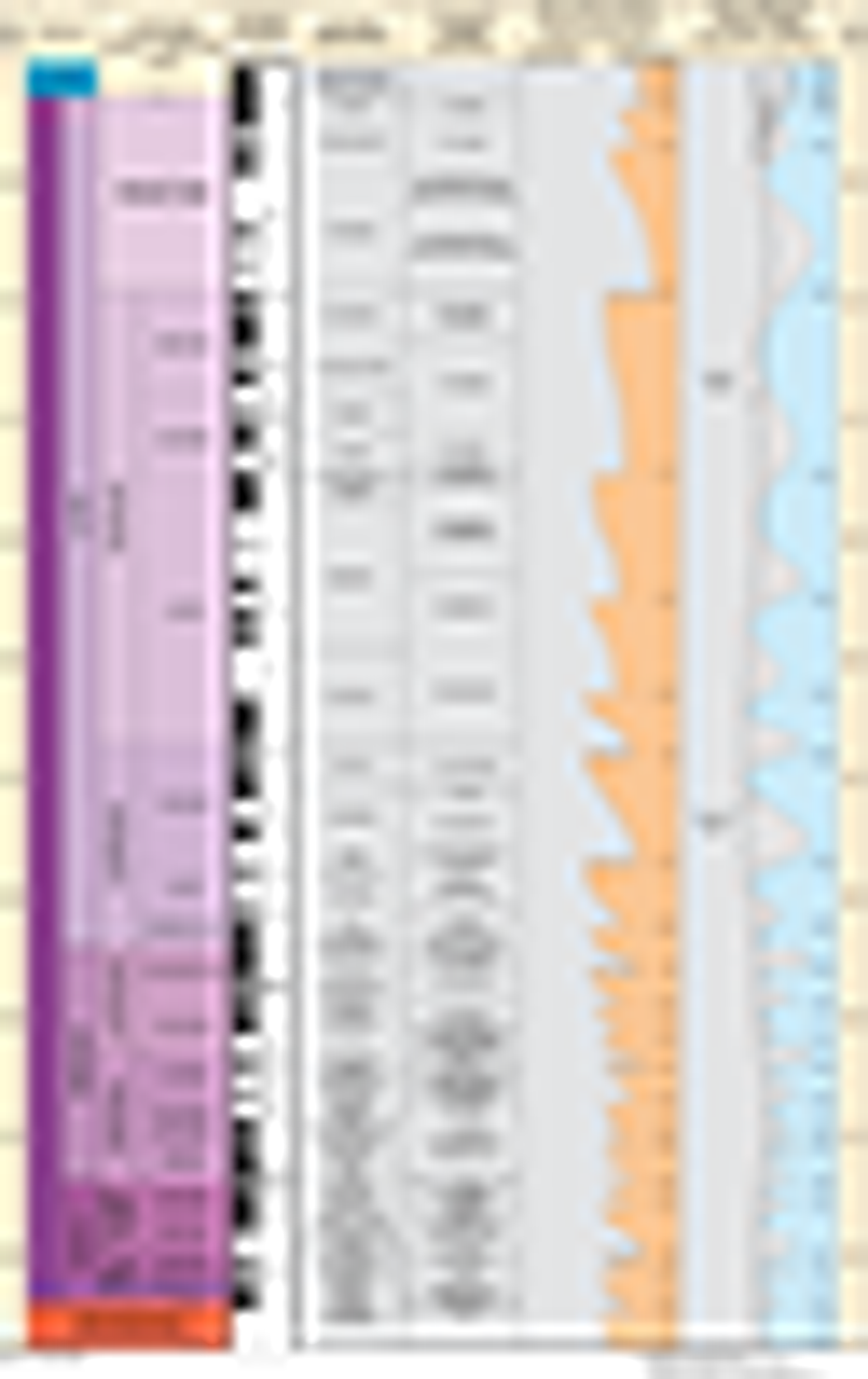
Triassic sequences and variations of sea level. Time scale after Ogg et al. (2016). Biozone cross-correlations are after Hardenbol et al. (1998). Sequence boundaries (sea-level fall events) are redesignated following a numbering scheme suggested by Hardenbol et al. (1998), however, the letter T is prefixed to each designation for convenience to make the numbers unique and not to confuse them with similar numbers in other periods. (Two events, in the Norian and Rhaetian [TNo2 and TRh1] are included provisionally, pending documentation of more widespread occurrence.)
The long-term eustatic trend shows that at the dawn of Triassic sea levels were near or a few meters higher than the present-day mean sea level (pdmsl) and then rose only ~10–20 m in the Induan and Olenekian. The base level actually fell just below pdmsl in the Anisian, reserving this trend in the Fassanian substage of the early Ladinian when a steady rise is seen that culminated in the highest sea levels of the Triassic (~50 m above pdmsl) in the Tuvalian substage of the late Carnian. From this peak the trend reverses again to a long-term decline in the Lacian substage of the early Norian. Through the Alaunian and much of the Sevatian substages of the late Norian, the base level remained steady and very close to pdmsl. At the Norian-Rhaetian boundary the base level dips once again just below pdmsl, recovering for a short time in the mid-Rhaetian and then declining rapidly to almost 50 m below pdmsl in the latest Triassic and earliest Jurassic.
The short-term sea-level curve, superimposed on the long-term eustatic curve, is based on sequence boundaries that are consistently correlatable in several basins are therefore considered widespread. Two cycles, one each in the Norian and the Rhaetian (TNo2 at 222.5 Ma and TRh1 at 203.5 Ma), are included tentatively, pending their confirmation from other areas as being more widespread. The amplitudes of third-order cycles (measures of sea-level falls in meters) are particularly difficult to estimate. The estimates of sea-level falls are always relative to the preceding highstand, and their determination criteria can include such relative measure as thickness of the system tracks, bio- and lithofacies depth assessments, depth of incision of shelves (in case of type-1 sequences), and partial back-stripping (see Haq, 2014, for further discussion). In the cycle chart presented here (Fig. 1) they are averaged from stratigraphic estimates in several basins and should be considered best guesstimates. They are categorized into three groupings of sea-level falls: major (>75 m of fall relative to previous high), medium (25–75 m of relative fall), and minor (<25 m of relative fall). Most Triassic sea-level falls were apparently of medium to minor magnitudes. The six falls that exceeded the 75 m amplitude, and are therefore considered major, include TIn3 at 250 Ma; TAn4 at 242.1 Ma; TLa3 at 238 Ma; TCa2 at 233.5 Ma; TCa3 at 229 Ma; and TNo4 at 209.7 Ma.
One clear trend in the Triassic is the overall low seastands of this period. If one were to also include the lowstands on both ends of the Triassic, i.e., in the latest Permian (starting ca. 260 Ma) as well as the earlier Jurassic (ending ca. 180.5 Ma), it represents an interval of almost 80 m.y., when the sea levels were universally low and do not seem to have risen more than 50 m above pdmsl at the highest point (in the Carnian). This 80-m.y. period was also an interval when there is no known evidence of large continental glaciations anywhere in the higher latitudes. Such a long duration of oceanic withdrawal from the large landmass of Pangaea seems unique in the Phanerozoic Earth history and would have had important repercussions for global climates and biodiversity (see further discussion in the GSA data repository [see footnote 1]). These could potentially include the presence of large desert areas and widespread salinas in arid regions, extreme climates, especially in the continental interiors, high sea-surface temperatures, relatively flat equator-to-pole gradients, and sluggish surface circulation. Deeper circulation would be characterized by warm saline bottom waters with intermittent loss of vertical stratification leading to widespread anoxia. Tropical shallow marine areas during relative highs could be sites of carbonate and extensive evaporite deposition. Biodiversities would decline when summer temperatures exceeded a certain threshold both on land and at sea. A long period of lowstand and continuous high temperatures also mean a deficit of biologic evolutionary innovations, and evidence gathered by Triassic paleoclimatic and paleoceanographic studies confirms these paleoenvironmental consequences. Biodiversity was decimated at the end-Permian extinction event and, after the Early through Middle Triassic recovery, declined once again during the long interval of the Late Triassic (these issues are discussed in the GSA data repository [see footnote 1]). The Triassic paleoenvironmental scenarios demonstrate the close link between eustasy, climates, and biodiversity.
The driving mechanism for the third-order cyclicity in the Triassic remains unidentified, an interval characterized by exceptionally long sedimentary eustatic periodicities in the Middle and Late Triassic (~5-m.y./cycle on average for third-order sequences) and no evidence of widespread glaciation. However, the relatively moderate variations in third-order sea levels make it tempting to consider the possibility of changes driven by the transfer of water to and from land aquifers as a potential cause. Since the early suggestion by Hay and Leslie (1990) and Jacobs and Sahagian (1993) there has been considerable recent interest in this mechanism as a potential cause for eustatic changes (e.g., Föllmi, 2012; Wagreich et al., 2014; Wendler and Wendler, 2016; Sames et al., 2016). Nevertheless, this process is more attuned to explaining modest (20–30 m) input/sequestration of water from/to land groundwater aquifers (and to a much lesser extent, the lakes that contribute only a minute, almost unmeasurable, amount to the total) to the ocean on Milankovitch time scales (Hay and Leslie, 1990). In the Triassic the process seems counterintuitive as very dry periods on land coincide with lowstands of sea level when presumably continental interiors would tend toward depleted aquifers (and also lack large lakes). The reverse also seems to be the case; i.e., during the late Carnian Pluvial Episode, when the climates were wetter and characterized by a single third-order event, the long-term sea level was also relatively higher. Thus, if the process has to work in the Triassic, it would have to have been on the shorter, Milankovitch, time scales.
What solid-Earth tectonic controls could have potentially influenced the sea-level changes in the Triassic when the planet was characterized by a large supercontinent with no apparent major ice accumulations on land? Most of the recent insights into the understanding of tectonic influences on sea level (as measured locally) either try to explain it on very short time scales (isostatic response to elastic and viscous loading and unloading) or on the very long time scales of multiple millions of years (see discussions in Haq, 2014, 2017, and Cloetingh and Haq, 2015). These influences cannot account for the third-order cyclicity in the Early and Middle Triassic (average duration of ~1 m.y./cycle in the Early and ~1.4 m.y./cycle in the Middle Triassic). However, for the multiple million-year cycles of the Late Triassic (average of ~3.6 m.y./cycle, but as large as ~7 m.y. for the longest Triassic cycle in late Norian), we may want to look for explanations in dynamic topographic effects that try to explain long-wavelength and long-term tectonic warping (see, e.g., Gurnis, 1993; Flament et al., 2013). On these longer scales subducting slabs underneath continents dramatically influence surface topography that in turn could drive local eurybathic sea-level changes. Thus, dynamic topography-driven variations seem to be a promising avenue to follow to explain the relatively small amplitude but long duration highs and lows (within the range of –50 m to +50 m of pdmsl) of the long-term eustatic sea level in the Triassic. So far such modeling for the Triassic supercontinent and its margins has not been attempted and is obviously an area of important future investigation.
Acknowledgments
The author is indebted to professors James Ogg, William Hay, Jerry Dickens, and an anonymous reviewer for detailed reviews of the paper and many useful suggestions that improved the quality of the paper. Christopher Scotese provided the reconstructions on which Figure S1 is based. Alexandre Lethier (Sorbonne, ISTEP) assiduously drafted the Triassic cycle chart presented in this paper and the figures in the GSA data repository that accompanies the paper.
References
- Aigner, T., and Bachmann, G., 1992, Sequence stratigraphic framework of the German Triassic: Sedimentary Geology, v. 80, p. 115–135, https://doi.org/10.1016/0037-0738(92)90035-P.
- Bhargava, O., Krystyn, L., Balini, M., Lein, R., and Nicora, A., 2004, Revised Litho- and Sequence Stratigraphy of the Spitin Triassic: Albertiana, v. 30, p. 21–39.
- Bourquin, S., Peron, S., and Durand, M., 2006, Lower Triassic sequence stratigraphy of the western part of the Germanic Basin (west Black Forest): Fluvial system evolution through time and space: Sedimentary Geology, v. 186, p. 187–211, https://doi.org/10.1016/j.sedgeo.2005.11.018.
- Budai, T., and Haas, J., 1997, Triassic sequence stratigraphy of the Balaton Highland, Hungary: Acta Geologica Hungarica, v. 40, no. 3, p. 307–335.
- Cloetingh, S., and Haq, B.U., 2015, Inherited landscapes and sea level change: Science, v. 347, https://doi.org/10.1126/science.1258375.
- Davies, J.H., Marzoli, A., Bertrand, H., Youbi, N., Ernesto, M., and Schaltegger, U., 2017, End- Triassic mass extinction started by intrusive CAMP activity: Nature Communications, https://doi.org/10.1038/ncomms15596.
- Embry, A.F., 1997, Global sequence boundaries of the Triassic and their identification in the Western Canada Sedimentary Basin: Bulletin of Canadian Petroleum Geology, v. 45, no. 4, p. 415–433.
- Flament, N., Gurnis, M., and Mueller, R. D., 2013, A review of observations and models of dynamic topography: Lithosphere, v. 5, p. 189–210, https://doi.org/10.1130/L245.1.
- Föllmi, K., 2012, Early Cretaceous life, climate and anoxia: Cretaceous Research, v. 35, p. 230–257, https://doi.org/10.1016/j.cretres.2011.12.005.
- Glørstad-Clark, E., Faleide J-I., Lunschien, B. and Nystuen, J., 2010, Triassic sequence stratigraphy and paleogeography of the western Barents Sea: Marine and Petroleum Geology, v. 27, p. 1448–1475, https://doi.org/10.1016/j.marpetgeo .2010.02.008.
- Gorter, J.D., 1994, Triassic sequence stratigraphy of the Carnarvon Basin, Western Australia in Purcell, P.G., and Purcell, R.R., eds., The Sedimentary Basins of Western Australia: Perth, Proceedings of the Petroleum Exploration Society Australia Symposium p. 397–413.
- Gurnis, M., 1993, Phanerozoic marine inundation of continents driven by dynamic topography above subducting slabs: Nature, v. 364, p. 589–593, https://doi.org/10.1038/364589a0.
- Haas, J., and Budai, T., 1999, Triassic sequence stratigraphy of the Transdanubian Range (Hungary): Geologica Carpathica, v. 50, no. 6, p. 459–475.
- Hallam, A., and Wignall, P.B., 1997, Mass extinctions and their aftermath: New York, Oxford University Press, 330 p.
- Haq, B.U., 2014, Cretaceous eustasy revisited: Global and Planetary Change, v. 113, p. 44–58, https://doi.org/10.1016/j.gloplacha.2013.12.007.
- Haq, B.U., 2017, Jurassic sea level variations: A reappraisal: GSA Today, v. 28, no. 1, doi:10.1130/GSATG359A.1.
- Haq, B.U., and Al-Qahtani, A.M., 2005, Phanerozoic cycles of sea-level change on the Arabian Platform: GeoArabia, v. 10, no. 2, p. 127–160.
- Haq, B.U., and Schutter, S.R., 2008, A chronology of Paleozoic sea-level changes: Science, v. 322, p. 64–68, https://doi.org/10.1126/science.1161648.
- Haq, B.U., Hardenbol, J., and Vail, P.R., 1987, Chronology of fluctuating sea level since the Triassic: Science, v. 235, p. 1156–1167, https:// doi.org/10.1126/science.235.4793.1156.
- Haq, B.U., Hardenbol, J., and Vail, P.R., 1988, Mesozoic and Cenozoic chronostratigraphy and cycles of sea-level change: Society of Economic Paleontologists and Mineralogists Special Publication, v. 42, p. 71–108.
- Hardenbol, J., Thierry, J., Farley, M.B., Jacquin, T., De Graciansky, P.C., and Vail, P.R., 1998, Mesozoic and Cenozoic sequence chronostratigraphic framework of European basins: Society of Economic Paleontologists and Mineralogists Special Publication 60, p. 3–13 (Chart 8, Triassic Chronostratigraphy).
- Hay, W.W., and Leslie, M.A., 1990, Could possible changes in global groundwater reservoir cause eustatic sea level fluctuations?, in Geophysics Study Committee, Mathematics and Resources, National Research Council, eds., Sea Level Change: Studies in Geophysics: Washington D.C., National Academy Press, p. 161–170.
- Jacobs, D.K., and Sahagian, D.L., 1993, Climate induced fluctuations in sea level during nonglacial times: Nature, v. 361, p. 710–712, https:// doi.org/10.1038/361710a0.
- Krystyn, L., Balini, M., and Nicora, A., 2005, Lower and Middle Triassic Stage and Substage Boundaries in Spiti, in Raju, D.S.D., Peters, J., Shanker, R., and Kumar, G., eds., An overview of litho-bio-chrono-sequence stratigraphy and sea level changes of Indian sedimentary basins: Association of Petroleum Geologists Special Publication 1, p. 66–74.
- Marzoli, A., Renne, P., Piccirillo, E., Bellieni, G., and De Min, A., 1999, Extensive 200-million year old continental flood basalts of the Central Atlantic magmatic province: Science, v. 284, p. 616–618, https://doi.org/10.1126/science .284.5414.616.
- Marzoli, A., Bertrand, H., Knight, K.B., Cirilli, S. Buratti, N., Vérati, C., Nomade, S., Renne, P.R., Youbi, N., Martini, R., Allenbach, K., Neuwerth, R., Rapaille, C., Zaninetti, L., and Bellieni, G., 2004, Synchrony of the Central Atlantic magmatic province and the Triassic- Jurassic boundary climatic and biotic crisis: Geology, v. 32, no. 11, p. 973–976, https:// doi.org/10.1130/G20652.1.
- Maurer, F., Rettori, R., and Martini, R., 2008, Triassic stratigraphy and evolution of the Arabian shelf in the northern United Arab Emirates: International Journal of Earth Sciences, v. 97, p. 765–784, https://doi.org/10.1007/s00531-007-0194-y.
- McElwain, J.C., Beerling, D., and Woodward, F., 1999, Fossil plants and global warming at Triassic-Jurassic boundary: Science, v. 285, 1386–1390, https://doi.org/10.1126/science.285.5432.1386.
- Mørk, A., Embry, A.F., and Weitschat, W., 1989, Triassic transgressive-regressive cycles in the Sverdrup Basin, Svalbard and the Barents Shelf, in Collinson, J.D., ed., Correlation in Hydrocarbon Exploration: Dordrecht, Springer, p. 113–130, https://doi.org/10.1007/978-94-009-1149-9_11.
- Ogg, J.G., Huang, C., and Hinnov, L., 2014, Triassic timescale status: A brief overview: Albertiana, v. 41, p. 3–30.
- Ogg, J.G., Ogg, G., and Gradstein, F.M., 2016, A Concise Geologic Time Scale: Amsterdam, Elsevier, 240 p.
- Preto, N., Kustatscher, E., and Wignall, P.B., 2010, Triassic climate—State of the art and perspectives: Palaeogeography, Palaeoclimatology, Palaeoecology, v. 290, p. 1–10, https://doi.org/ 10.1016/j.palaeo.2010.03.015.
- Raup, D.M., and Sepkowski, J., Jr., 1982, Mass extinctions in the marine fossil record: Science, v. 215, p. 1501–1503, https://doi.org/10.1126/ science.215.4539.1501.
- Sames, B., Wagreich, M., Wendler, J., Haq, B., Conrad, C., Melinte-Dobrinescu, M., Hu, X., Wendler, I., Wolfgring, E., Yilmaz, I., and Zorina, S., 2016, Review: Short-term sea-level changes in a greenhouse world—A view from the Cretaceous: Palaeogeography, Palaeoclimatology, Palaeoecology, v. 441, p. 393–411, https:// doi.org/10.1016/j.palaeo.2015.10.045.
- Sharland, P.R., Archer, R., Casey, D.M., Davies, R.B., Hall, S.H., Heward, A.P., Horbury, A.D., and Simmons, M.D., 2001, The chrono-sequence stratigraphy of the Arabian Plate: GeoArabia Special Publication 2, 371 p.
- Sharland, P.R., Casey, D.M., Davies, R.B., Simmons, M.D., and Sutcliffe, O.E., 2004, Arabian plate sequence stratigraphy—Revisions to SP2: GeoArabia, v. 9, no. 1, p. 199–214.
- Sun, Y., Joachimski, M., Wignall, P.B., Yan, C., Chen, Y., Jiang, H., Wang, L., and Lai, X., 2012, Lethally hot temperatures during the early Triassic greenhouse: Science, v. 338, p. 366–370, https://doi.org/10.1126/science.1224126.
- Tong, J., and Yin, H., 1998, The marine Triassic sequence stratigraphy of Lower Yangtze: Science in China, v. 41, no. 3, p. 255–261, https:// doi.org/10.1007/BF02973113.
- Trotter, J.A., Williams, I.S., Nicora, A., Mazza, M., and Rigo, M., 2015, Long-term cycles of Triassic climate change: A new delta 18O record from conodont apatite: Earth and Planetary Science Letters, v. 415, p. 165–174, https://doi.org/10.1016/ j.epsl.2015.01.038.
- van der Meer, D.G., van Saparoea, A., van Hinsbergen, D., van de Weg, R., Godderis, Y., Le Hir, G., and Donnadieu, Y., 2017, Reconstructing first-order changes in sea level during the Phanerozoic and Neoproterozoic using strontium isotopes: Gondwana Research, v. 44, p. 22–34, https://doi.org/10.1016/j.gr.2016.11.002.
- van Veen, P.M., Skojld, L.J., Kristensen, S.E., Rasmussen, A., Gjelberg, J., and Stølen, T., 1992, Triassic sequence stratigraphy in the Barents Sea, in Vorren, T.O., Bergsager, E., Dahl-Stamnes, O.A., Holter, E., Johansen, B., Lie, E., and Lund, T.B., eds., Arctic Geology and Petroleum Potential: NPF Special Publication, v. 2, p. 515–538.
- von Rad, U., Thurow, J., Haq, B.U., Gradstein, F., Ludden, J., and the ODP Leg 122/123 Shipboard Scientific Parties, 1989, Triassic to Cenozoic evolution of the NW Australian continental margin and birth of the Indian Ocean (preliminary results of ODP Legs 122 & 123): Geologische Rundschau, v. 78, p. 1189, https://doi.org/10.1007/BF01829340.
- Wagreich, M., Lein, R., and Sames, B., 2014, Eustasy, its controlling factors, and the limnoeustatic hypothesis—Concepts inspired by Eduard Suess: Journal of Austrian Earth Science, v. 107, no. 1, p. 115–131.
- Wendler, J.E., and Wendler, I., 2016, What drove cyclic sea-level fluctuations during the mid- Cretaceous greenhouse climate?: Palaeogeography, Palaeoclimatology, Palaeoecology, v. 441, p. 412–419, https://doi.org/10.1016/j.palaeo .2015.08.029.