
Full Text View
Volume 27 Issue 2 (February 2017)
GSA Today
![]()
Article, pp. 4-10 | Abstract | PDF (556KB)
Impact of seismic image quality on fault interpretation uncertainty
Cover Image
Table of Contents
- Introduction
- How Do We See Seismic Images?
- Interpretation Experiment
- Image Analysis
- Interpretation Outcomes
- Image Quality
- Impact on Interpretation
- Acknowledgments
- References Cited
Search GoogleScholar for
Search GSA Today
Abstract
Uncertainty in the geological interpretation of a seismic image is affected by image quality. Using quantitative image analysis techniques, we have mapped differences in image contrast and reflection continuity for two different representations of the same grayscale seismic image, one in two-way-time (TWT) and one in depth. The contrast and reflection continuity of the depth image is lower than that of the TWT image. We compare the results of 196 interpretations of a single fault with the quality of the seismic image. Low contrast and continuity areas correspond to a greater range of interpreted fault geometries, resulting in a broader spread of fault interpretations in the depth image. Subtle differences in interpreted fault geometries introduce changes in fault characteristics (e.g., throw, heave) that are critical for understanding crustal and lithospheric processes. Seismic image quality impacts interpretation certainty, as evidenced by the increased range in fault interpretations. Quantitative assessments of image quality could inform: (1) whether model-based interpretation (e.g., fault geometry prediction at depth) is more robust than a subjective interpretation; and (2) uncertainty assessments of fault interpretations used to predict tectonic processes such as crustal extension.
*Current address: Cardiff University School of Earth and Ocean Sciences, Main Building, Park Place, Cardiff, CF10 3AT, UK.
**E-mails: juan.alcalde@abdn.ac.uk, clare.bond@abdn.ac.uk, g.johnson@ed.ac.uk, ellisj11@cardiff.ac.uk, rob.butler@abdn.ac.uk
Manuscript received 3 Feb. 2016; Revised manuscript received 8 Apr. 2016; Accepted 6 July 2016; Posted online 9 Jan. 2017
Introduction
Interpreting seismic reflection data is the principal approach for obtaining a detailed understanding of the geological structure of the subsurface. Central to these endeavors is the ability to trace faults. The resulting interpretations of fault patterns are used to infer a wide variety of tectonic properties—for example: estimations of upper crustal stretching during lithospheric extension (e.g., Kusznir and Karner 2007); kinematic connectivity and stretching directions (e.g., Baudon and Cartwright, 2008); and polyphase reactivation and inversion (e.g., Underhill and Paterson, 1998; Badley and Backshall, 1989). Fault interpretations are important components in the prediction of hydrocarbon reservoir volumes in structural traps, and in forecasting the integrity and performance for structurally complex reservoirs (e.g., Richards et al., 2015; Yielding, 2015; Wood et al., 2015; Freeman et al., 2015). However, in publications, faults are commonly shown as single, deterministic interpretations—even though there are uncertainties in these seismic interpretations that will impact the application of the interpretation. A single seismic image can comprise a range of interpretations with intrinsic probabilities (Bond et al., 2007; Hardy, 2015). Despite the importance of fault interpretations, remarkably few publications or indeed training materials explain how faults are interpreted on seismic reflection profiles or discuss the uncertainties in the interpretations. Here we explore how image quality impacts fault interpretation, using outputs from an interpretation exercise.
Faults may be characterized as quasi-planar features that offset geological markers. It is rare that the fault surfaces themselves generate seismic reflections. Therefore, on seismic images, fault geometries are established chiefly by linking the terminations of stratal reflectors (e.g., Bahorich and Farmer, 1995). However, there are many other explanations for reflector termination, some geophysical (e.g., noise, processing effects, anomalous changes in velocity) and some geological (e.g., depositional facies changes, channels, unconformities), that are not always easy to distinguish, so there are ambiguities in fault interpretation. Subtle differences in fault interpretation introduce changes in the geometric characteristics of the faults (e.g., throw, heave), with, for example, impact on the determination of stretching factors for sedimentary basins. For basins in a late stage of being explored, 3D seismic data are often employed because they generally provide a higher spatial resolution and geometric continuity compared with even closely spaced grids of 2D seismic profiles (Cartwright and Huuse, 2005; Gao, 2009), but there can still be significant uncertainty in structural interpretation. Regardless of the development of 3D seismic methods, 2D data continue to underpin regional tectonic studies and frontier basin exploration (e.g., Platt and Philip, 1995; Thomson and Underhill, 1999; Gabrielsen et al., 2013). Much of the understanding of fault geometry is based on heritage 2D data from the 1980s (e.g., Freeman et al., 1990), even if enhanced by subsequent 3D studies (e.g., Cartwright and Huuse, 2005). Furthermore, training materials in fault interpretation (e.g., Shaw et al., 2005), as well as knowledge-sharing resources (i.e., books and articles), are chiefly two-dimensional, presented in paper or on computer screen. In summary, 2D interpretation is a fundamental and important part of most seismic interpretations irrespective of whether the data are available as 2D lines or 3D volumes. In spite of its importance, the impression given by these training materials and by the expert community is that fault interpretation in seismic imagery is routine and carries little uncertainty.
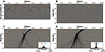 Figure 1
Seismic sections used in the interpretation experiment. (A) Seismic section in two-way travel time (TWT). (B) Seismic section in depth. (C) and (D) stacked results of the interpreted faults in TWT and depth (respectively). The figure includes the histogram of the corresponding section. In the histograms, the x-axis represents the possible gray values (from 0-black to 255-white) and the y-axis the number of pixels found for each value. Note that the sections conserve the vertical scale in which they were presented to the participants and that the results in TWT were converted to depth, to be comparable with those interpreted in the depth section. The sections are courtesy of BP/GRUPCO. Q1 and Q3—first and third quartiles.
How Do We See Seismic Images?
Seismic data are viewed and interpreted manually as images. There are a number of visual factors that affect how we perceive objects, including color, intensity, hue, and perspective (e.g., Froner et al., 2013). These factors determine the saliency of the different elements that form an image. Visual saliency refers to the distinctiveness of an element; i.e., the capacity to draw the attention of the viewer (e.g., Kadir and Brady, 2001; Kim et al., 2010), and is mainly dependent on its distinction from nearby elements (Cheng et al., 2011). Visual saliency produces biases in favor of the most prominent elements (Reynolds and Desimone, 2003), and hence influences interpretation. As such, increasing image contrast enhances differences between prominent elements in an image (Reynolds and Desimone, 2003).
Classically, seismic imagery is presented as a grayscale, although it is now commonly visualized in color, using either linear or nonlinear color spectrums (Froner et al., 2013). Nonlinear color spectrums are often used to highlight maximum and minimum amplitude reflectors. When employing an 8-bit black-and-white computer render, image contrast represents the range in amplitude of seismic reflection data as 256 pixels in different shades of gray. Similarly, reflection continuity (the saliency of a reflector) is represented by adjoining pixels of the same, or a similar, shade of gray. Modern 64-bit computers can display images in millions of gray or color shades. However, human perception of images presented in gray scale is poorly understood and an active area of research (Song et al., 2010; Radonjić et al., 2011). Our aim is to test if even “simple” 8-bit grayscale visualizations of seismic images of different quality have an impact on interpretation outcome.
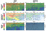 Figure 2
Results of the analysis carried out in two-way travel time (TWT) (A, C, and E) and depth (B, D, and F) seismic sections with the respective fault spread superimposed (outlier limits marked with dashed lines; quartiles 1 and 2 marked in continuous lines). (A) and (B) contrast analysis—warm colors represent high values in interquartile difference (i.e., high contrast) and cold colors represent low values (i.e., low contrast). (C) and (D) continuity analysis—reflections colored according to the length of their major axis, with warm colors indicating long lengths (i.e., high continuity) and cold colors short length (i.e., low continuity). (E) and (F) merge of the two analyses—the results have been combined in a 1:1 relation; that is, the contrast and continuity values have been multiplied and normalized to 100. Note that the TWT results have been depth-converted for comparison (i.e., located at the same point) to the depth results. The black lines at the left side of the images mark the depths of the nine positions at which the fault placement for the interpretation populations was computed in each seismic image.
Interpretation Experiment
We presented a seismic image to 196 interpreters in a controlled experiment and compared their interpretations of a major fault in the seismic image with the image quality. The seismic reflection image from the Gulf of Suez (Fig. 1) was presented either in two-way travel time (TWT, Fig. 1A)—70 subjects, 36% of the interpretations—or in depth domain (Fig. 1B)—126 subjects, 64% of the interpretations (Figs. 1C and 1D, respectively). The participants were asked to “interpret the major fault crossing the section and the main sedimentary horizons as deep as they could.” They were also asked to provide further annotation and/or sketching to support their interpretations. In this contribution, we focus purely on the fault interpretations as drawn by the participants on the seismic image. Participants had up to 30 minutes to complete their interpretations. The interpreters’ proficiencies were highly diverse, and their experience ranged from unexperienced students to interpretation specialists with more than 30 years of experience.
The seismic section used in the experiment was 31 km long and extended to 6 s TWT (Fig. 1A). The seismic image included a lateral disruption of the reflections in the central part, generally interpreted as a fault, but with some degree of uncertainty as to the fault’s placement, geometry, and extent. The TWT section was converted to depth using a simple velocity model in MoveTM, described by Equation (1):
![]() (1)
(1)
where Z is the depth in meters, V0 is the initial velocity (1500 ms−1), t is one-way travel time, and k is the rate of change in velocity with increasing depth (0.5). The depth conversion located the bottom of the section at 10.5 km depth. The depth conversion was completed on a bitmap of the seismic reflection image, which linearly stretches the image. The result is a depth section with apparently lower reflectivity and contrast than the original TWT image and 18% longer, due to this stretching. With the exception of depth conversion, both the TWT and depth images share identical processing workflows. The actual depth conversion method used is not important for our experiment; it is the difference in image quality the process creates that concerns us.
Image Analysis
The image analysis undertaken focused on the pixel intensity contrast and reflection continuity (referred to hereafter as “contrast” and “continuity,” respectively) of the TWT and depth sections (see Fig. S1 in GSA’s Supplemental Data Repository1). For the image analysis, each seismic image was subdivided into cells of 7.2 km (length) × 1 km (depth) (1135 × 450 pixels). The area encompassing the participants’ fault interpretations was subdivided into smaller cells, 1.6 km × 0.4 km (216 × 163 pixels), in order to provide detailed image analysis information in the area of interest. For ease of comparison of our results, the seismic images are both shown with a vertical scale in depth in all figures (except Fig. 1A).
To analyze the image contrast we extracted grayscale distributions for the pixels in each cell for the two uninterpreted images. The distributions range from pixel number 0 (black) to 255 (white): the wider these distributions are (i.e., the more pixel values close to the extremes of 0 and 255), the more contrast the image has; the narrower the pixel distribution, the more similar the pixel values are and thus the lower the contrast. The first and third quartiles (Q1 and Q3) from these distributions were subtracted in order to calculate the interquartile range (IQ) of the distributions. We use the interquartile range as an analogue for visual contrast: the wider the IQ of the cell, the higher the contrast and vice versa. Each cell in the images is colored according to its IQ value in order to display graphically the contrast analysis results.
To analyze the reflector continuity, the images were first converted into a binary, i.e., a black and white image. This was performed using ImageJ software (Schneider et al., 2012) by setting an automatic threshold level based on the histograms of the two images. This threshold divides the pixel histogram in two halves, assigning black or white color to all the pixels. As a result, the seismic wave reflections are separated into isolated black bodies, corresponding to the positive amplitude reflections in this particular case, included in a white background. A macro for the software ImageJ (Heilbronner and Barrett, 2013) was used to measure and analyze these resultant bodies. In the analysis, the length of the major axis of each reflection is calculated, using a best-fit ellipse method, and each reflection is then colored based on this length value using a color scale.
Interpretation Outcomes
Interpretations of the major discontinuity of reflectors (faults) located in the middle of the seismic images and related splay faults (327 elements in total) were used in the analysis. Of these elements, 116 correspond to the interpretations of the TWT image (Fig. 1C) and 211 to the interpretations of the depth seismic image (Fig. 1D). In general, variability in fault placement position (the spread in fault interpretations) increases with depth, and this observation is more pronounced in those interpretations derived from the depth image. The difference in fault placement spread between the two images is at a maximum at 5 km depth. Below this point, the amount of interpreted faults dipping to the right is greater in the depth section (23 faults) than in the TWT section (5 faults). The effect of the difference in the populations of TWT and depth interpretations was analyzed by randomly selecting 70 of the depth interpretations for comparison with the TWT interpretation population of 70. Because these were found to be similar to the full-depth interpretation analysis, we conclude that the population size had no effect on the results.
Quantification of the variability in fault placement for the interpretation populations were computed at nine depth markers in each seismic image (Fig. 2). The four quartile and outlier positions for the fault interpretation populations were calculated at each depth marker (results of the analysis are shown in Fig. 2, overlying the image analyses). The interquartile fault range (the distance between the first and third quartiles) provides a good estimation of the fault placement spread within each of the interpretation populations at a given depth (continuous black lines in Fig. 2, created from joining the quartiles between depth markers). We use the interquartile range of fault placement within each fault interpretation population as an indicator of fault placement uncertainty for each seismic image. The interquartiles show that fault spread remains similar in the upper 3.5 km. From 3.5 km downward, the interquartile fault range in the depth image increases until, at the base of the seismic image, the interquartile width is twice that observed in the TWT image. The increase in fault spread defined by the interquartile trend linearly increases in the TWT image with depth. In the depth image, the first quartile follows a similar path to that of the TWT image, but the third quartile is more heterogeneous (wavy) and is offset to the right with respect to the third quartile line in the TWT image. Meanwhile, the outliers (dashed black lines in Fig. 2) show a similar general pattern with fault spread increasing with depth, but with a greater variability and heterogeneity. The fault placement outliers for the fault interpretations of the TWT image show a convergent trend down to 2 km in width at ~4 km depth before the fault placement spread increases to ~15 km at the base of the image. The fault placement outliers from the depth interpretation show a relatively constant spread (~4.5 km width) down to 3 km depth. Below this point, fault spread increases with depth, resulting in a 15-km spread in fault interpretations at the base of the seismic image. There is also a clear difference in the length of the faults interpreted. The depth of the first and last point of the faults were measured, resulting in an average depth of 4.7 km and 6.6 km for the faults interpreted in TWT and depth, respectively.
Image Quality
Image Contrast
Contrast in the TWT seismic image is almost three times greater than in the depth image (Figs. 1C and 1D). Detailed contrast analysis of both seismic images shows a decrease in contrast with depth as well as higher contrast to the left of the fault location as compared to the right (Figs. 2A and 2B). There is a visible spatial association between lower contrast areas in the seismic imagery and a larger spread in fault placement certainty (Figs. 2A and 2B). This effect is especially visible in areas with very low IQ, which correspond to maximum fault placement dispersion (i.e., dark green and blue colors in Fig. 2B). In the TWT seismic image, the IQ values remain moderate when compared to the depth image. This may account for the smaller interquartile range in fault placement in the lower half of the TWT image in comparison to the depth image (Fig. 2B).
The outlier fault interpretations (dashed lines in Figs. 2A and 2B) are also likely to have been affected by image contrast; indications of this influence can be seen in Figure 2A, where the left outlier line follows the yellow/green pixel contrast binning boundary at 2.5–7 km depth. The convexity of the right outlier toward the third quartile at 3.5 km depth and ~15 km distance along the TWT seismic image was associated with the existence of higher contrast cells (yellow colors) in comparison to surrounding cells at this point (Fig. 2A).
Reflection Continuity
Reflection continuity decreases with depth in the seismic images and to the right of the main fault. Reflection continuity is, on average, 63% smaller in the depth image than in the TWT image (Figs. 2C and 2D). We associate this dramatic reduction in continuity to the decrease in contrast as a result of the depth conversion. Interpreted faults tend to cross areas with lower reflection continuity. This is not surprising, because faults that cut and disrupt rock layers with the same reflective physical properties would create low reflection continuity. The fault interpretations coincide with where reflectors from the left join those coming from the right, at ~13–16 km along the seismic image, at ~6 km depth. The third quartile of the TWT interpretations follow this boundary. In the depth seismic image this joining of reflectors is less clear (potentially due to the lack of reflectivity/continuity), and the third quartile is more variable, especially in the deeper part below 5 km. The greater amount of faults dipping to the right below 5 km depth in the depth image can be explained by a lack of reflection continuity at distances along the section line >13 km, and 5 km depth (Fig. 2D). In the TWT image, right-dipping faults have to be interpreted crossing strong, continuous reflections below 5 km, and most right-dipping fault interpretations stop at shallower depths (from 17 fault interpretations at 3 km depth to only 5 at 5 km depth). In the depth image, the reflections are more discontinuous and fault interpretations continue to greater depths. The extent of the outliers also seems to be affected by reflection continuity. In the TWT seismic image for example, the right outlier line coincides with a break in reflection continuity between 4–10 km depth (Fig. 2C); in the depth image, the right outlier stays to the left of a package with more continuous horizontal reflections, located at 2.5–5.5 km depth (Fig. 2D).
Combined Image Analysis
The analysis of contrast and continuity highlighted spatial associations between image quality and fault interpretation (Figs. 2A–2D). In reality, the image, as viewed by the interpreter, is the result of combining both contrast and continuity. In an attempt to merge the results of the contrast and continuity analyses, the continuity analysis was converted into a cell model, based on the contrast grid. This conversion assigned the maximum continuity value contained within a cell to each cell in the grid. To merge the analyses, cells in the new continuity cell model were multiplied with the values from the respective cells from the contrast analysis. In spite of the potential different impact of the two parameters on the interpreters and their relative co-dependency (i.e., enhancing the contrast can enhance the continuity), creating a combined parameter provides a general visualization of image quality. The results were normalized by representing the maximum value as 100 and the minimum as zero. The resulting merged models for the depth-converted TWT and depth images are shown in Figures 2E and 2F.
There is a diffuse horizontal boundary in the merged values in the TWT image at ~4.5 km depth (Fig. 2E), marking a change from “green” and hotter colors at shallower levels to lower “blue” values as depth increases. This 4.5 km depth marks the point at which the distance between the first and third quartiles increases from 523 m to more than double (1234 m) at the bottom of the section. This boundary also coincides with the average depth of the interpreted TWT faults, suggesting that it marks a clear increment in the uncertainty of the image for interpretation. Faults are interpreted until a deeper point in the depth image, potentially because this boundary in image quality is less perceptible. The positions of the outlier interpretations show a greater change, from a narrow converging spread to divergent with the spread increasing with depth. In the case of the depth image (Fig. 2F), this boundary is less noticeable, possibly due to the overall low values and poor image quality, although fault spread does increase with depth below 4.5 km. The results suggest that there may be a contrast and continuity threshold within the seismic images beyond which the fault interpretations are almost unconstrained by the data.
Impact on Interpretation
The experiment outlined above shows that image contrast and the continuity of features both impact on the interpretation outcome of the seismic imagery. Interpreters are less prone to cross stratal reflections if they are “strong” (i.e., high contrast and high continuity), and where reflections are “weak,” uncertainty in interpretation increases. In general, enhancing image contrast helps to constrain the interpretation, as seen in the TWT image, where image contrast is three times that of the depth image and the fault placement population shows a narrower spread and shorter faults. A similar pattern is observed for reflection continuity, where high reflection continuity also results in a narrower fault placement spread and shorter fault interpretations. The differences in fault spread observed determine predicted fault heave, resulting, for example in regional sections, in significant differences in crustal stretching predictions. Further work to assess the relative contributions of contrast and continuity to visual image quality to create a single weighted parameter would provide a fully quantified visualization of image quality.
The two images were presented in different domains (TWT and depth), resulting in an 18% longer vertical scale in the depth image that could have changed the perception of the fault geometries to interpreters. However, our correlations suggest that image quality had the major influence on interpretation choice. We note that the average depth of the faults interpreted in the TWT image coincides with a boundary in depreciating image quality in the combined analysis. Although our results show that depth conversion choices (including the method used) change seismic image quality, all image manipulations have the potential to change interpretation outcomes. We therefore need to better understand image perception so that such image manipulations do not arbitrarily influence or bias interpretation outcome.
For a fixed binary threshold, image contrast and continuity are associated parameters, so increasing image contrast can artificially increase continuity. This correlation causes issues in determining the best methods for enhancing imagery in order to maximize interpretation effectiveness. It also has impacts on the processing of seismic data and the model chosen to create an image. Initial processing models generally assume a sub-horizontal, sub-parallel reflector stratigraphy with minimal disruption. Thus, they enhance reflector continuity. Our results, albeit based on TWT and depth imagery rather than different processing models, show that reflector continuity is spatially related to fault placement certainty. The processing of strong reflector continuity in seismic image data may result in greater constraint, or certainty, in fault placement than is warranted by the original data. Processing models must therefore be chosen carefully and interaction between the processor and the interpreter encouraged.
The results of the image analysis imply that there is a threshold at which seismic image data are too indeterminate (i.e., not enough contrast or continuity) to drive the interpretation. Quantitative image analysis could be used to determine the extent of an interpretation that is data-supported and areas that are more subjective. To create interpretations for under-constrained problems, reference models, such as fold or fault shape, can be employed. These reference models can be based on mechanical and geometric rules: e.g., angle of faulting, based on Andersonian mechanics (Anderson, 1905, 1951), or depth to detachment for faults (Chamberlin, 1910), based on mass balance principles (Dahlstrom, 1969; Elliott, 1983). Indeed, Bond et al. (2012) show that in areas of poor constraint, simple geological reasoning and reconstruction analysis can be used to reduce interpretation uncertainty. The method proposed in this work opens the door for a workflow for image quality assessment to indicate those occasions when model-based interpretation (e.g., fault geometry prediction at depth) may be more robust than the subjective fault interpretation of a geologist. Of course, these two approaches are complementary: image analysis may aid the interpreter in determining when geometric modeling may be useful and when interpretation uncertainty, and therefore potential risk, is high.
Even in the advent of more complex visualization through computing and screen technology, including the use of color and a greater pixel spectrum, interpretation uncertainty is determined by the quality of a seismic image. Understanding the impact of image quality on seismic interpretation using an 8-bit grayscale image provides a basis from which to investigate more complex aspects of visual perception, including color and luminescence. This work requires interdisciplinary research with cognitive scientists, neurologists, and others to fully understand how best to represent seismic imagery to maximize interpretation efforts.
A key finding of our experiments is that there are significant variations in the interpretation of fault geometries as depth increases in the section. This reflects the decay in image quality with depth. This uncertainty may be important—for example in picking the hanging-wall cut-offs of stratal reflectors on normal faults to correlate with those in the footwall that are otherwise well-imaged. This, in turn, influences determinations of fault heave—information that is critical for constructing maps that show fault linkages in sedimentary basins and for determining net extension of the upper crust. These inherent uncertainties arising from image quality are generally unreported in larger-scale studies of fault patterns. Therefore, the maps and net extension calculations used in many tectonic studies carry unknown errors.
Acknowledgments
BP/GUPCO are acknowledged for providing data from the Gulf of Suez. The authors acknowledge the support of MVE and use of Move software 2015.2 for this work. Ruediger Kilian is acknowledged for his kind help with the ImageJ code. Dr. Juan Alcalde is funded by NERC grant NE/M007251/1, on interpretational uncertainty. The work could not have been completed without the support of individuals within the geoscience community who took part in the interpretation experiment.
References Cited
- Anderson, E.M., 1905, The dynamics of faulting: Transactions of the Edinburgh Geological Society, v. 8, p. 387–402, doi: 10.1144/transed.8.3.387.
- Anderson, E.M., 1951, The Dynamics of Faulting and Dyke Formation with Application to Britain, Second Edition: Edinburgh, Oliver and Boyd, 206 p.
- Badley, M.E., and Backshall, L.C., 1989, Inversion, reactivated faults and related structures: Seismic examples from the southern North Sea, in Cooper, M.A., and Williams, G.D., eds., Inversion Tectonics: Geological Society, London, Special Publication 44, p. 201–219, doi: 10.1144/GSL.SP.1989.044.01.12.
- Bahorich, M., and Farmer, S., 1995, 3-D seismic discontinuity for faults and stratigraphic features: The coherence cube: The Leading Edge, v. 14, no. 10, p. 1053–1058, doi: 10.1190/1.1437077.
- Baudon, C., and Cartwright, J., 2008, The kinematics of reactivation of normal faults using high resolution throw mapping: Journal of Structural Geology, v. 30, no. 8, p. 1072–1084, doi: 10.1016/j.jsg.2008.04.008.
- Bond, C.E., Gibbs, D., Shipton, Z.K., and Jones, S., 2007, What do you think this is? “Conceptual uncertainty” in geoscience interpretation: GSA Today, v. 17, no. 11, p. 4–10, doi: 10.1130/GSAT01711A.1.
- Bond, C.E., Lunn, R.J., Shipton, Z.K., and Lunn, A.D., 2012, What makes an expert effective at interpreting seismic images?: Geology, v. 40, no. 1, p. 75–78, doi: 10.1130/G32375.1.
- Cartwright, J., and Huuse, M., 2005, 3D seismic technology: The geological “Hubble”: Basin Research, v. 17, no. 1, p. 1–20, doi: 10.1111/j.1365-2117.2005.00252.x.
- Chamberlin, R.T., 1910, The Appalachian folds of central Pennsylvania: The Journal of Geology, v. 18, p. 228–251, doi: 10.1086/621722.
- Cheng, M.-M., Zhang, G.-X., Mitra, N.J., Huang, X., and Hu, S.-M., 2011, Global contrast based salient region detection: Proceedings of the IEEE Computer Society Conference on Computer Vision and Pattern Recognition, article no. 5995344, p. 409–416.
- Dahlstrom, C.D.A., 1969, Balanced cross sections: Canadian Journal of Earth Sciences, v. 6, p. 743–757, doi: 10.1139/e69-069.
- Elliott, D., 1983, The construction of balanced cross-sections: Journal of Structural Geology, v. 5, p. 101.
- Freeman, B., Yielding, G., and Badley, M., 1990, Fault correlation during seismic interpretation: First Break, v. 8, no. 3, p. 87–95.
- Freeman, B., Quinn, D.J., Dillon, C.G., Arnhild, M., and Jaarsma, B., 2015, Predicting subseismic fracture density and orientation in the Gorm Field, Danish North Sea, in Richards, F.L., Richardson, N.J., Rippington, S.J., Wilson, R.W., and Bond, C.E., eds., Industrial Structural Geology: Principles, Techniques and Integration: Geological Society, London, Special Publication 421, p. 421–429.
- Froner, B., Purves, S.J., Lowell, J., and Henderson, J., 2013, Perception of visual information: The role of colour in seismic interpretation: First Break, v. 31, no. 4, p. 29–34.
- Gabrielsen, P.T., Abrahamson, P., Panzner, M., Fanavoll, S., and Ellingsrud, S., 2013, Exploring frontier areas using 2D seismic and 3D CSEM data, as exemplified by multi-client data over the Skrugard and Havis discoveries in the Barents Sea: First Break, v. 31, no. 1, p. 63–71.
- Gao, D., 2009, 3D seismic volume visualization and interpretation: An integrated workflow with case studies: Geophysics, v. 74, no. 1, p. W1–W12, doi: 10.1190/1.3002915.
- Hardy, S., 2015, The devil truly is in the detail. A cautionary note on computational determinism: Implications for structural geology numerical codes and interpretation of their results: Interpretation (Tulsa), v. 3, no. 4, p. SAA29–SAA35, doi: 10.1190/INT-2015-0052.1.
- Heilbronner, R., and Barrett, S., 2013, Image Analysis in Earth Sciences: Microstructures and Textures of Earth Materials: Springer Science & Business Media, v. 129, 513 p.
- Kadir, T., and Brady, M., 2001, Saliency, scale and image description: International Journal of Computer Vision, v. 45, no. 2, p. 83–105, doi: 10.1023/A:1012460413855.
- Kim, Y., Varshney, A., Jacobs, D.W., and Guimbretiere, F., 2010, Mesh saliency and human eye fixations. ACM Transactions on Applied Perception, v. 7, no. 2, Article 12, February 2010, 13 pages, doi: 10.1145/1670671.1670676.
- Kusznir, N.J., and Karner, G.D., 2007, Continental lithospheric thinning and breakup in response to upwelling divergent mantle flow: Application to the Woodlark, Newfoundland and Iberia margins, in Karner, G.D., Manatschal, G., and Pinheiro, L.M., eds., Imaging, Mapping and Modelling Continental Lithosphere Extension and Breakup: Geological Society, London, Special Publication 282, p. 389–419, doi: 10.1144/SP282.16.
- Platt, N.H., and Philip, P.R., 1995, Structure of the southern Falkland Islands continental shelf: Initial results from new seismic data: Marine and Petroleum Geology, v. 12, no. 7, p. 759–771, doi: 10.1016/0264-8172(95)93600-9.
- Radonjić, A., Allred, S.R., Gilchrist, A.L., and Brainard, D.H., 2011, The dynamic range of human lightness perception: Current Biology, v. 21, no. 22, p. 1931–1936, doi: 10.1016/j.cub.2011.10.013.
- Reynolds, J.H., and Desimone, R., 2003, Interacting roles of attention and visual salience in V4: Neuron, v. 37, no. 5, p. 853–863, doi: 10.1016/S0896-6273(03)00097-7.
- Richards, F.L., Richardson, N.J., Bond, C.E., and Cowgill, M., 2015, Interpretational variability of structural traps: Implications for exploration risk and volume uncertainty, in Richards, F.L., Richardson, N.J., Rippington, S.J., Wilson, R.W., and Bond, C.E., eds., Industrial Structural Geology: Geological Society, London, Special Publication 421, p. 7–27.
- Schneider, C.A., Rasband, W.S., and Eliceiri, K.W., 2012, NIH Image to ImageJ: 25 years of image analysis: Nature Methods, v. 9, p. 671–675, doi:10.1038/nmeth.2089.
- Shaw, J.H., Connors, C., and Suppe, J., eds., 2005, Seismic interpretation of contractional fault-related folded: Tulsa, Oklahoma, AAPG Seismic Atlas: Studies in Geology, v. 53, p. 156.
- Song, M., Tao, D., Chen, C., Li, X., and Chen, C.W., 2010, Color to gray: Visual cue preservation: IEEE Transactions on Pattern Analysis and Machine Intelligence, v. 32, no. 9, p. 1537–1552, doi: 10.1109/TPAMI.2009.74.
- Thomson, K., and Underhill, J.R., 1999, Frontier exploration in the South Atlantic: Structural prospectivity in the North Falkland Basin: AAPG Bulletin, v. 83, no. 5, p. 778–797.
- Underhill, J.R., and Paterson, S., 1998, Genesis of tectonic inversion structures: Seismic evidence for the development of key structures along the Purbeck-Isle of Wight Disturbance: Journal of the Geological Society, v. 155, no. 6, p. 975–992, doi: 10.1144/gsjgs.155.6.0975.
- Wood, A.M., Paton, D.A., and Collier, R.E.L., 2015, The missing complexity in seismically imaged normal faults: What are the implications for geometry and production response? in Richards, F.L., Richardson, N.J., Rippington, S.J., Wilson, R.W., and Bond, C.E., eds., Industrial Structural Geology: Geological Society, London, Special Publication 421, p. 213–230.
- Yielding, G., 2015, Trapping of buoyant fluids in fault-bound structures, in Richards, F.L., Richardson, N.J., Rippington, S.J., Wilson, R.W., and Bond, C.E., eds., Industrial Structural Geology: Geological Society, London, Special Publication 421, p. SP421–SP423.