An open-source software environment for visualizing and refining plate tectonic reconstructions using high-resolution geological and geophysical data sets
Simon E. Williams, R. Dietmar Müller, Thomas C.W. Landgrebe, Joanne M. Whittaker
In this article
Full Text View
Volume 22 Issue 4 (April/May 2012)
GSA Today
Article, pp. 4-9 | Abstract | PDF (3.5MB)
An open-source software environment for visualizing and refining plate tectonic reconstructions using high-resolution geological and geophysical data sets
[Table: Table of Contents Introduction The Next Generation of Plate Reconstruction Software Reconstruct...]
Simon E. Williams*, R. Dietmar Müller, Thomas C.W. Landgrebe, Joanne M. Whittaker*
Earthbyte Group, School of Geosciences, Madsen Building F09, University of Sydney, Sydney NSW 2006, Australia
Abstract
We describe a powerful method to explore spatio-temporal relationships within geological and geophysical data sets by analyzing the data within the context of tectonic reconstructions. GPlates is part of a new generation of plate reconstruction software that incorporates functionality familiar from GIS software with the added dimension of geological time. Here we use GPlates to reconstruct geological terranes, geophysical grids, and paleomagnetic data within alternative tectonic models of the assembly of Western Australia and the configuration of Rodinia. With the ability to rapidly visualize a diverse range of geological and geophysical constraints within different reconstructions, users can easily investigate the implications of different tectonic models for reconciling a variety of observations and make more informed choices between different models and data.
*Email:
Manuscript received 23 Sept. 2011; accepted 7 Feb. 2012.
DOI: 10.1130/GSATG139A.1
Introduction
Geoscientists have come to rely strongly on computing technology. Until a few decades ago, geological maps and cross sections were assembled on paper. Now, Geographic Information System (GIS) software has revolutionized the way we store and work with geospatial data (Whitmeyer et al., 2010). It is now possible to rapidly integrate vast arrays of geoscientific data into single digital maps that enable complex present-day spatial relationships to be explored and understood. Within a GIS, we can interactively add data, modify symbologies, arrange data into layers, and create and modify interpretations. At the same time, geoscientists are cognizant that the data they are collecting and analyzing has reached its present-day location as a result of complex tectonic histories—there are often important spatio-temporal relationships between samples that are now far apart but that were once much more proximal to each other.
Plate tectonic models have implications for geoscientists in a wide range of disciplines—fields as diverse as determining the geodynamic controls on arc-magmatism (e.g., Straub et al., 2009) and ore deposit formation; modeling the evolution of ocean current circulation (e.g., Berggren and Hollister, 1977); understanding the global fossil record by identifying pathways for species migration (e.g., Ali and Aitchison, 2008); and interpreting the signatures in mantle seismic tomography images (e.g., van der Meer et al., 2010). They all invoke plate kinematic models to support their hypotheses.
A notable early illustration of plate tectonics was presented in the continental drift “flipbook” of Scotese (1976). Since then, animations illustrating the relative motions of Earth’s tectonic plates over geological time scales have become widely available. However, these animations are essentially a series of static images—maps that cannot be modified or interacted with—and the ability for users to incorporate their own data or images into the plate tectonic animation has remained largely elusive. Suppose we have a plate tectonic animation for an area that we are studying and for which we have additional data sets. How can we relate our own data (which contain information about geological events but are expressed in their present-day locations) to the plate configuration and motions at the time of these events? Such a scenario illustrates the need for tools combining the functionality typical of GIS software with the capability to quickly and easily reconstruct and visualize geospatial data back through time. Therefore, there is a need for a tool that loads geospatial data, whether in point, vector, or raster format (akin to standard GIS software), and then visualizes these data in their plate tectonic context based on available plate motion models and time-varying properties. Additionally, such software should enable users to develop and modify their own plate models.
The Next Generation of Plate Reconstruction Software
To respond to these needs, the past decade has seen the development of several tools for tectonic reconstruction. Some of these tools are proprietary software for commercial use, aimed, for example, mainly at understanding the formation of petroleum and ore deposit systems in a paleogeographic context. For the wider scientific community, there are several publically available (and in some cases open source) plate tectonic softwares (e.g., GMAP, Torsvik and Smethurst, 1999; PaleoMac, Cogné, 2003; PLACA, Matias et al., 2005; PPlates, Smith et al., 2007), some of which have a specific emphasis on the analysis of paleomagnetic data in a plate tectonic context or on plate deformation.
Here, we describe GPlates, part of a new generation of software tools enabling geoscientists from a broad range of disciplines to work with plate tectonic models and efficiently link these models to their own data. GPlates software (Boyden et al., 2011; Gurnis et al., 2012), an open-source, cross platform Geographic Information System (GIS), was developed in collaboration with the University of Sydney, the California Institute of Technology, and the Geological Survey of Norway. It is a virtual globe in the same manner as Google Earth, with the added dimension of geological time, thus enabling 4-D visualizations to refine and improve the quality of tectonic reconstruction. Importantly, GPlates can reconstruct a wide variety of data types, including high-resolution geophysical images, which is of particular importance for optimizing and critically assessing plate motion models. All figures in this paper were created using GPlates.
The following is a typical workflow using GPlates to easily load and reconstruct data and then create custom animations of the reconstruction (see footnote 1 for a link to more detailed step-by-step instructions):
1 All figures in this paper were created using freely available data and software. The data sets used to make Figures 3 and 4, as well as a more detailed GPlates tutorial, are provided in appendices S1–S2 at ftp.earthbyte.org/earthbyte/GSA_Today_2012. GPlates is open-source, cross-platform software available at www.gplates.org.
- Load vector data into GPlates. Point, line, and polygon data can be loaded into GPlates. Currently, a number of prevalent formats for the transfer of GIS and geoscientific vector data can be loaded (and written), including ESRI shapefiles and open standards-based XML formats such as GML (Geographic Markup Language) and GeoSciML (GeoSciML, 2011). GPlates incorporates support for a native XML-based format called GPML (GPlates Markup Language), based on GML, and provides direct access to data available through Web Feature Services.
- Load raster data into GPlates. Raster data can be loaded into GPlates either as an image file (.jpg, .png, etc.) or as a netCDF grid. These input raster files/images may cover the entire globe or part of the globe (see the Australian use-case described in a following section).
- “Cookie-cut” data. All loaded data can be attached to a plate-tectonic reference with a few simple steps via an underlying plate model so that the data are assigned to the appropriate plates and reconstructed accordingly. Plate models typically comprise a global set of polygons, which define the extent of each of Earth’s tectonic plates. Any loaded vector or raster data can be “cookie-cut” based on these plate definitions; subsequently, each vector or raster fragment is reconstructed individually according to a selected reconstruction model.
For areas of oceanic crust, reconstructed rasters are progressively masked based on the crustal age at the pixel location using a grid of ocean floor age (Müller et al., 2008). - Reconstruct and explore data. Once prepared, data sets (including rasters) can be continuously reconstructed on-the-fly backward and forward in time. This is made possible by taking advantage of desktop graphics hardware via the OpenGL programming interface, where an innovative approach has been used to map spherical spatial data into graphics constructs. The vast majority of desktop graphics hardware manufactured in the last decade is more than capable of displaying raster data at interactive frame rates, provided that culling and level-of-detail techniques are employed to reduce the CPU workload. High-resolution images are decomposed into sets of tiles at several levels of resolution so that the highest resolution images are only used when the zoom level is high.
- Export reconstructed data, images, and animations. Snapshots of reconstructed data can be exported from GPlates in a number of vector (shapefiles, SVG, GMT ASCII) and raster (e.g., .jpg, .tif) formats for a variety of uses, such as creating figures for publications and animations for presentations.
Reconstructing Supercontinents
Plate tectonic software is only useful if we have—or want to create—realistic models for Earth’s plate tectonic evolution. For the Cretaceous and Tertiary periods, models based primarily on ocean-floor magnetic and fracture zone data are now well constrained for most of the ocean basins, and several global-scale models (Müller et al., 2008; Torsvik et al., 2008; Schettino and Scotese, 2005) have been published. Our supplementary material (see footnote 1) includes an example of reconstructing data within Pangea using publically available global plate models.
Figures 1 and 2 illustrate reconstructing data within the supercontinent Rodinia, one of Pangea’s predecessors. A range of plate tectonic models has been proposed for the assembly and subsequent breakup of Rodinia during the Meso- to Neo-proterozoic. Compared to reconstructions of Pangea, alternative Rodinia models differ widely in their basic characteristics, both at the global scale (e.g., Pisarevsky et al., 2003; Li et al., 2008; Evans, 2009) or in terms of the fit of individual continents. For example, there is considerable debate over Proterozoic connections between Laurentia, Australia, and Antarctica—models include the SWEAT model linking the Southwestern United States to East Antarctica (e.g., Dalziel, 1997); the AUSWUS model linking Australia to the Southwestern United States (e.g., Karlstrom et al., 1999); and the AUSMEX model linking Australia to Mexico (Wingate et al., 2002).
Figure 1
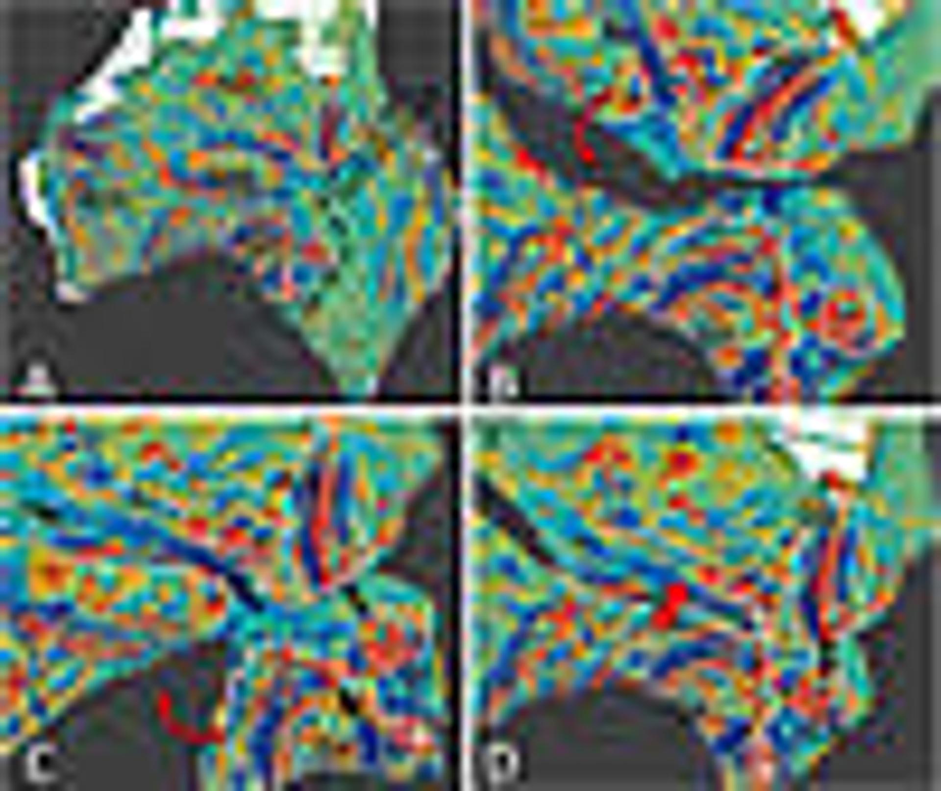
Screenshots of reconstructions generated in GPlates, geological vector data loaded into three different proposed scenarios for the configuration of Laurentia, Australia, and East Antarctica ca. 780 Ma. The data displayed are areas of outcropping Precambrian rocks (Bouysse, 2010, pink polygons) and Proterozoic large igneous provinces from Ernst et al. (2008—colored by age): (A) SWEAT (poles of rotation from Dalziel, 1997); (B) AUSWUS (poles of rotation from Karlstrom et al., 1999); (C) AUSMEX (poles of rotation from Wingate et al., 2002).
Figure 2
Plate tectonic reconstruction in GPlates at 780 Ma, following two contrasting models for the configuration of Rodinia: (A) is based on the block definitions and poles of rotation of Li et al. (2008); (B) uses the same block definitions but the poles of rotation of Evans (2009). The data are the world magnetic anomaly map (EMAG2, Maus et al., 2009). Coastlines are shown in black; cratonic block boundaries are shown in white.
Reconstructions for these times rely on a diverse range of data sets. Paleomagnetic data can provide constraints on the paleo-latitudes and relative rotations between adjacent continental blocks (e.g., Evans, 2009). Further evidence can be accumulated via correlation of geological signatures between continents, such as the alignment of linear trends of basement terranes interpreted from geophysical and geological mapping and matching ages and/or geochemical signatures of magmatism. Integrating all these data is not trivial but can be simplified and made accessible to a wider community of geoscientists through plate tectonic modeling software. Figure 1 shows how GPlates can be used to quickly reconstruct the same geological data within alternative reconstruction models. The figure shows the distribution of large igneous provinces formed during the Meso- and Neoproterozoic, digitized based on a shapefile from Ernst et al. (2008) and reconstructed following the SWEAT, AUSWUS, and AUSMEX scenarios.
Geophysical images are another important constraint on these reconstructions. Aeromagnetic data have been used to constrain tectonic reconstructions at various scales, including constraining the relative position of Australia and Antarctica using satellite magnetics (Goodge and Finn, 2010); the evolution of an early Paleozoic volcanic arc (Greenfield et al., 2010); Proterozoic tectonics within Australia (Aitken and Betts, 2008); and displacements across individual faults (Cather et al., 2006). For reconstructing ancient continents, continuous data coverage allows the extent and fabric of mapped basement units to be extended beneath more recent cover rocks (Finn and Pisarevsky, 2007). In Figure 2, we show the global crustal magnetic anomaly map EMAG2 (Maus et al., 2009). These data are loaded into GPlates as a georeferenced .jpg, then reconstructed within two alternative global models for the configuration of Rodinia ca. 780 Ma—the models of Li et al. (2008) and Evans (2009).
Figures 1 and 2 illustrate striking differences between alternative Rodinia interpretations. Our supplemental material (see footnote 1) includes a tutorial explaining how to load, reconstruct, and interact with such data. Next, we focus on a regional example—the Proterozoic evolution of Australia. This allows us to make use of the much higher resolution magnetic anomaly compilation available for this continent.
A Use Case—The Proterozoic Evolution of Australia
While eastern Australia is composed of a series of Phanerozoic accretionary belts, areas of the Australian continent to the west of the so-called “Tasman Line” (Direen and Crawford, 2003) (Fig. 3A) have been relatively stable throughout the Phanerozoic. However, continent-scale geological structures provide evidence for earlier major tectonic events related to relative motions between ancient cratonic blocks that comprise the western two- thirds of Australia.
Figure 3
(A) Reduced-to-pole magnetic anomalies for Australia. The North, South, and West Australian cratons are labeled NAC, SAC, and WAC respectively. MB—Musgrave Block (see text). (B–D) Magnetic data reconstructed using three candidate plate configurations proposed for Australia since the early Mesoproterozoic (ca. 1600 Ma): (B) after Li and Evans (2011), a 40° rotation of NAC; (C) Giles et al. (2004), 52° rotation of SAC; (D) after Henson et al. (2011), translation of NAC relative to WAC and SAC. White outlines show the Curnamona Province (Cu) and Mount Isa Block (MI), Arunta Inlier (Ar) and Gawler craton (Ga); these are discussed in the text (adapted from Cawood and Korsch [2008]). The graticule interval is 10°.
The older parts of Australia are generally described in terms of the North, West, and South Australian cratons (Myers et al., 1996), from here on abbreviated to NAC, WAC, and SAC, respectively (see Fig. 3A and supplementary material [footnote 1]). These cratons are separated by younger (Neoproterozoic to early Paleozoic) orogenic belts. To piece together the basic crustal evolution of Australia during the Proterozoic, we need to establish how these three blocks have moved relative to one another (as well as the other blocks within Rodinia) and at what point they assembled into the configuration we see today.
A recent study by Li and Evans (2011) proposes a 40° rotation of the NAC relative to the SAC and WAC. The rotation is interpreted from paleomagnetic data, which indicate that relative motion postdates 750 Ma. In their present-day configuration, the NAC and SAC/WAC are separated by units of the Petermann and Paterson Orogens, a ca. 600–530 Ma intracontinental tectonic event (Raimondo et al., 2010) interpreted to involve significant convergence and dextral shear between the NAC and SAC/WAC. Li and Evans (2011) suggest that, prior to the Neoproterozoic rotation, the relative NAC/WAC juxtaposition may have persisted since 1800 Ma.
Such a model has implications for the alignment of any geological structures between the two blocks (NAC and SAC/WAC) that predate the rotation. A number of authors have emphasized the similarities in the age and geochemical compositions of Paleoproterozoic units within the Mount Isa Block on the NAC and the Broken Hill Inlier within the Curnamona province on the SAC (e.g., Giles et al., 2004). Presently, Mount Isa and Broken Hill lie >1000 km apart, and some authors have argued that these provinces were more closely juxtaposed during the geodynamic events that formed these units. For example, Giles et al. (2004) juxtapose Mount Isa and Curnamona prior to 1300 Ma by invoking a 52° rotation of the SAC relative to the NAC/WAC. In this model, the NAC and WAC are assumed to be fixed together in their present-day configuration from ca. 1700 Ma onward, in contrast to the Li and Evans (2011) interpretation. Alternatively, translation (without relative rotation) of the NAC relative to the SAC could restore Curnamona toward Mount Isa—for example, by invoking a 600-km, NE-SW sinistral strike-slip displacement (Wilson, 1987) or broadly N-S translation (Henson et al., 2011), implying subsequent net extension between the NAC and SAC.
Each of these models makes testable predictions. The relative rotation should result in lateral offsets between older geological features that were previously adjacent and/or aligned. Reconstructing geological and geophysical data that describe these features allows us to evaluate different tectonic scenarios much more effectively than if we simply view all of these ancient structures in their present-day configuration.
Figure 3 shows magnetic data reconstructed using the different proposed reconstruction scenarios for Proterozoic Australia. Here we have used the fifth edition of the magnetic anomaly map for Australia (Milligan et al., 2010). The data have been reduced to the pole (RTP) using a variable magnetic inclination RTP algorithm to remove the latitude dependence of the induced anomaly shapes (P.R. Milligan, 2011, personal commun.). The reconstructed configurations of Giles et al. (2004) and Henson et al. (2011) bring into closer juxtaposition the distinctive anomaly patterns in the Mount Isa and Curnamona Province regions. The Li and Evans (2011) model (Fig. 3B) leaves Mount Isa and Curnamona widely separated (instead, the regional lineation trend of anomalies in the Mount Isa region broadly aligns with regional anomaly trends between the SAC and WAC, possibly related to the Mesoproterozoic Albany Fraser Orogen). The magnetic anomalies also reveal the structural grain within the Gawler craton and Arunta Inlier. Giles et al. (2004) argue that these two provinces formed a continuous orogenic belt along Australia’s southern margin during the late Paleoproterozoic. Figure 3C illustrates how the rotation of the SAC yields continuity in the grain of the magnetic anomalies between the Gawler and Arunta provinces (cf. figure 4 in Giles et al., 2004). By comparison, the magnetic fabric between these provinces appears less continuous within the reconstruction of Li and Evans (2011).
Next, we explore the paleomagnetic data available to constrain these models. Schmidt et al. (2006) analyzed available paleomagnetic data for volcanic rocks from ca. 1070 Ma, including parts of the Warakurna Large Igneous Province, with sample sites distributed across the SAC, NAC, and WAC. Figure 4 shows the virtual geomagnetic poles from ca. 1070 Ma used by Li and Evans (2011)—one from the WAC (the Bangemall Sills) and two from the NAC (from the Stuart Dikes and Alcurra Dikes respectively—the latter lying on the Musgrave Block, assumed to be part of the NAC since this time). These poles are important lines of evidence for their interpretation and are clearly better aligned with their proposed rotation of the NAC, whereas the model of Giles et al. (2004) does not attempt to reconcile these data. We also plot an additional pole used by Schmidt et al. (2006) for the Gawler Dikes on the SAC, originally taken from Giddings and Embleton (1976). This pole is not used by Li and Evans (2011), possibly because the Gawler Dikes from which the pole is derived are not directly dated—rather, the age is inferred by Schmidt et al. (2006) from nearby volcanic rocks that have been dated. If this inference is correct and the paleopole is reliable, then the configuration shown in Figure 4 would need to be further revised to reconcile this additional constraint. Schmidt et al. (2006) conclude that each of the three ancient Australian cratonic blocks may have had independent polar wander paths throughout the Paleo- and Mesoproterozoic and did not reach their final assembly until after the Warakurna event.
Figure 4
Plate tectonic reconstruction in GPlates for 1070 Ma. The configuration of Rodinia is taken from the model of Li et al. (2008), with additional motion between the North, South, and West Australian cratons (NAC and SAC/WAC) based on Li and Evans (2011). The rotation of the NAC proposed by Li and Evans to occur ca. 600 Ma reconciles paleomagnetic data for the NAC and WAC (green and cyan) at 1070 Ma; however, this model does not reconcile these poles with an additional pole from the SAC (purple) used by Schmidt et al. (2006). The reconstruction is shown in a fixed West Australia reference frame. The graticule interval is 10°.
Many other data sets can provide clues to the Proterozoic configuration of Australia. In the supplementary material (see footnote 1), we include an additional geological data set to accompany the Australia use case—age-code polygons representing the extent of different Proterozoic mafic-ultramafic magmatic events generated by Geoscience Australia (Claoué-Long and Hoatson, 2009). Many of these magmatic events predate the various proposed block motions we discussed earlier, so the configurations in Figure 3 represent candidates for the crustal configuration at the time of this magmatism.
Conclusions and Implications
The broader aim of this article is to illustrate the way geoscientists can use plate tectonic modeling software to critically evaluate existing reconstructions, better understand their own data within the context of these models, identify correlations or inconsistencies between different data sets, and ultimately generate more robust geological interpretations. To make such software relevant to a wide range of geoscientists, the software needs to be accessible and contain functionality that allows workers to easily load and interrogate their data. Cutting up and reconstructing raster data can be achieved to some extent using computer software that allows image manipulation or by simply printing an image and cutting it up with scissors. However, performing these tasks within plate modeling software has a number of advantages:
- Within a GIS environment, with a series of images and vector data as layers, we can apply a candidate plate motion and immediately see its consequences for all the neighboring plates and data sets involved.
- The data are positioned on a spherical Earth, and rotated shapes are not distorted.
- Plate modeling software like GPlates can also be used to modify existing models or to create new plate tectonic models from scratch. Such software can easily determine the Euler poles of rotation that describe the best-fitting reconstructions, save them to use again, distribute these models to colleagues, and publish them.
Our discussion has concentrated on what has recently become possible within GPlates, such as the visualization and rapid reconstruction of large vector and raster data sets in a GIS-like environment. In the future, the enormous growth of digital data sets, the increasing detail of plate tectonic models, and the diversity of both spatial data types and their respective subcommunities call for systematic, quantitative workflows and methodologies.
As a simple, freely available software package, GPlates has applications beyond pure research problems. It is already used as a teaching tool to facilitate learning about Earth’s geological history and processes. Visualizations created in GPlates provide a means for geoscientists to more effectively communicate the outcomes of their research to the general public.
Acknowledgments
We thank Peter Milligan of Geoscience Australia for providing the RTP magnetic data of the Australian continent. John Cannon helped to prepare the text, and the cover image associated with this paper was prepared by Sabin Zahirovic. Thanks also to editor R. Damian Nance and two anonymous reviewers for their valuable comments. S. Williams, R. Müller, and T. Landgrebe were supported by Australian Research Council grant FL0992245; J. Whittaker was supported by Statoil.
REFERENCES CITED
- Aitken, A.R.A., and Betts, P.G., 2008, High-resolution aeromagnetic data over central Australia assist Grenville-era (1300–1100 Ma) Rodinia reconstructions: Geophysical Research Letters, v. 35, L01306, 6 p., doi: 10.1029/2007GL031563.
- Ali, J.R., and Aitchison, J.C., 2008, Gondwana to Asia: Plate tectonics, paleogeography and the biological connectivity of the Indian sub-continent from the Middle Jurassic through latest Eocene (166–35 Ma): Earth-Science Reviews, v. 88, p. 145–166.
- Berggren, W.A., and Hollister, C.D., 1977, Plate tectonics and paleocirculation-commotion in the ocean: Tectonophysics, v. 38, p. 11–48.
- Bouysse, P., 2010, Geological Map of the World, Third Edition: Commission for the Geological Map of the World, scales: 1:50,000,000 and 1:25,000,000, http://ccgm.free.fr/index_gb.html (last accessed 9 Feb. 2012).
- Boyden, J.A., Müller, R.D., Gurnis, M., Torsvik, T.H., Clark, J.A., Turner, M., Ivey-Law, H., Watson, R.J., and Cannon, J.S., 2011, Next-generation plate-tectonic reconstructions using GPlates, in Keller G.R., and Baru, C., eds., Geoinformatics: Cyberinfrastructure for the Solid Earth Sciences: Cambridge, UK, Cambridge University Press, p. 95–114.
- Cather, S., Karlstrom, K., Timmons, J., and Heizler, M., 2006, Palinspastic reconstruction of Proterozoic basement-related aeromagnetic features in north-central New Mexico: Implications for Mesoproterozoic to late Cenozoic tectonism: Geosphere, v. 2, p. 299–323, doi: 10.1130/GES00045.1.
- Cawood, P.A., and Korsch, R.J., 2008, Assembling Australia: Proterozoic building of a continent: Precambrian Research, v. 166, p. 1–38.
- Claoué-Long, J.C., and Hoatson, D.M., 2009, Guide to using the Map of Australian Proterozoic Large Igneous Provinces: Geoscience Australia, record 2009/44, 37 p.
- Cogné, J., 2003, PaleoMac: A Macintosh application for treating paleomagnetic data and making plate reconstructions: Geochemistry, Geophysics, Geosystems, v. 4, 1007, 8 p., doi: 10.1029/2001GC000227.
- Dalziel, I.W.D., 1997, Neoproterozoic-Paleozoic geography and tectonics: Review, hypothesis, environmental speculation: GSA Bulletin, v. 109, p. 16–42, doi: 10.1130/0016-7606(1997)109<0016:ONPGAT>2.3.CO;2.
- Direen, N.G., and Crawford, A., 2003, The Tasman Line: Where is it, what is it, and is it Australia’s Rodinian breakup boundary?: Australian Journal of Earth Sciences, v. 50, p. 491–502.
- Ernst, R.E., Wingate, M.T.D., Buchan, K.L., and Li, Z.X., 2008, Global record of 1600–700 Ma Large Igneous Provinces (LIPs): Implications for the reconstruction of the proposed Nuna (Columbia) and Rodinia supercontinents: Precambrian Research, v. 160, no. 1–2, p. 159–178.
- Evans, D.A.D., 2009, The palaeomagnetically viable, long-lived and all-inclusive Rodinia supercontinent reconstruction, in Murphy, J.B., Keppie, J.D., and Hynes, A.J., eds., Ancient Orogens and Modern Analogues: London, Geological Society Special Publication 327, p. 371–404, doi: 10.1144/SP327.16.
- Finn, C.A., and Pisarevsky, S., 2007, New airborne magnetic data evaluate SWEAT reconstruction, in Cooper, A.K., Raymond, C., and the 10th ISAES Editorial Team, eds., Antarctica: A Keystone in a Changing World—Online Proceedings of the 10th ISAES X: USGS Open-File Report 2007-1047, extended abstract 170, 4 p., http://pubs.usgs.gov/of/2007/1047/ea/of2007-1047ea170.pdf (last accessed 9 Feb. 2012).
- GeoSciML, 2011, Geoscience Markup Language: Commission for the Management and Application of Geoscience Information (CGI): http://www.geosciml.org/geosciml/2.0/doc/ (last accessed 9 Feb. 2012).
- Giddings, J., and Embleton, B., 1976, Precambrian palaeomagnetism in Australia II: Basic dykes from the Gawler Block: Tectonophysics, v. 30, p. 109–118.
- Giles, D., Betts, P.G., and Lister, G.S., 2004, 1.8–1.5-Ga links between the North and South Australian cratons and the Early-Middle Proterozoic configuration of Australia: Tectonophysics, v. 380, p. 27–41.
- Goodge, J.W., and Finn, C.A., 2010, Glimpses of East Antarctica: Aeromagnetic and satellite magnetic view from the central Transantarctic Mountains of East Antarctica: Journal of Geophysical Research, v. 115, B09103, 22 p., doi: 10.1029/2009JB006890.
- Greenfield, J., Musgrave, R., Bruce, M., Gilmore, P., and Mills, K., 2010, The Mount Wright Arc: A Cambrian subduction system developed on the continental margin of East Gondwana, Koonenberry Belt, eastern Australia: Gondwana Research, v. 19, p. 650–669, doi: 10.1016/j.gr.2010.11.017.
- Gurnis, M., Turner, M., Zahirovic, S., DiCaprio, L., Spasojevich, S., Müller, R.D., Boyden, J., Seton, M., Manea, V.C. and Bower, D., 2012, Plate reconstructions with continuously closing plates: Computers & Geosciences, v. 38, p. 35–42, doi: 10.1016/j.bbr.2011.03.031.
- Henson, P., Kositcin, N., and Huston, D., 2011, Broken Hill and Mount Isa: Linked but not rotated: Geoscience Australia, AUSGEO News, v. 102, p. 13–17.
- Karlstrom, K.E., Harlan, S.S., Williams, M.L., McLelland, J., Geissman, J.W., and Åhäll, K.-I., 1999, Refining Rodinia: Geologic evidence for the Australia–Western U.S. connection in the Proterozoic: GSA Today, v. 9, no. 10, p. 1–7, /gsatoday/archive/9/10/pdf/gt9910.pdf (last accessed 9 Feb. 2012).
- Li, Z.X., and Evans, D.A.D., 2011, Late Neoproterozoic 40° intraplate rotation within Australia allows for a tighter-fitting and longer-lasting Rodinia: Geology, v. 39, p. 39–42, doi: 10.1130/G31461.1
- Li, Z.X., Bogdanova, S., Collins, A.S., Davidson, A., De Waele, B., Ernst, R., Fitzsimons, I., Fuck, R., Gladkochub, D., and Jacobs, J., 2008, Assembly, configuration, and break-up history of Rodinia: A synthesis: Precambrian Research, v. 160, p. 179–210.
- Matias, L.M., Olivet, J.L., Aslanian, D., and Fidalgo, L., 2005, PLACA: A white box for plate reconstruction and best-fit pole determination: Computers & Geosciences, v. 31, no. 4, p. 437–452.
- Maus, S., Barckhausen, U., Berkenbosch, H., Bournas, N., Brozena, J., Childers, V., Dostaler, F., Fairhead, J., Finn, C., and von Frese, R., 2009, EMAG2: A 2-arc min resolution Earth Magnetic Anomaly Grid compiled from satellite, airborne, and marine magnetic measurements: Geochemistry, Geophysics, Geosystems, v. 10, Q08005, 12 p., doi: 10.1029/2009GC002471.
- Milligan, P.R., Franklin, R., Minty, B.R.S., Richardson, L.M., and Percival, P.J., 2010, Magnetic Anomaly Map of Australia (Fifth Edition): Canberra, Geoscience Australia, scale: 1:15,000,000, http://www.ga.gov.au/image_cache/GA18012.pdf (last accessed 9 Feb. 2012).
- Müller, R., Sdrolias, M., Gaina, C., and Roest, W., 2008, Age, spreading rates, and spreading asymmetry of the world’s ocean crust: Geochemistry, Geophysics, Geosystems, v. 9, Q04006, 19 p., doi: 10.1029/2007GC001743.
- Myers, J.S., Shaw, R.D., and Tyler, I.M., 1996, Tectonic evolution of Proterozoic Australia: Tectonics, v. 15, p. 1431–1446.
- Pisarevsky, S.A., Wingate, M.T.D., Powell, C.M.A., Johnson, S., and Evans, D.A.D., 2003, Models of Rodinia assembly and fragmentation, in Yoshida, M., Windley, B.E., and Dasgupta, S., eds., Proterozoic East Gondwana: Supercontinent Assembly and Breakup: London, Geological Society Special Publication 206, p. 35–55.
- Raimondo, T., Collins, A.S., Hand, M., Walker-Hallam, A., Smithies, R.H., Evins, P.M., and Howard, H.M., 2010, The anatomy of a deep intracontinental orogen: Tectonics, v. 29, TC4024, 31 p., doi: 10.1029/2009TC002504.
- Schettino, A., and Scotese, C.R., 2005, Apparent polar wander paths for the major continents (200 Ma to the present day): A palaeomagnetic reference frame for global plate tectonic reconstructions: Geophysical Journal International, v. 163, p. 727–759.
- Schmidt, P.W., Williams, G.E., Camacho, A., and Lee, J.K.W., 2006, Assembly of Proterozoic Australia: Implications of a revised pole for the 1070 Ma Alcurra Dyke Swarm, central Australia: Geophysical Journal International, v. 167, p. 626–634.
- Scotese, C., 1976, A continental drift ‘flip book’: Computers & Geosciences, v. 2, p. 113–116, doi: 10.1016/0098-3004(76)90096-0.
- Smith, M., Kurtz, J., Richards, S., Forster, M., and Lister, G., 2007, A re-evaluation
- of the breakup of South America and Africa using deformable mesh reconstruction software: Journal of the Virtual Explorer v. 25, p. 1–13.
- Straub, S.M., Goldstein, S.L., Class, C., and Schmidt, A., 2009, Indian-type mid-ocean ridge basalts in the northwest Pacific Ocean basin: Nature Geoscience, v. 2, p. 286–289.
- Torsvik, T.H., and Smethurst, M.A., 1999, Plate tectonic modeling: Virtual reality with GMAP: Computers & Geosciences, v. 25, p. 395–402, doi: 10.1016/S0098-3004(98)00143-5.
- Torsvik, T.H., Müller, R.D., van der Voo, R., Steinberger, B., and Gaina, C., 2008, Global plate motion frames: Toward a unified model: Reviews of Geophysics, v. 46, RG3004, 44 p., doi: 10.1029/2007RG000227.
- van der Meer, D.G., Spakman, W., van Hinsbergen, D.J.J., Amaru, M.L., and Torsvik, T.H., 2010, Towards absolute plate motions constrained by lower-mantle slab remnants: Nature Geoscience, v. 3, p. 36–40, doi: 10.1038/ngeo708.
- Whitmeyer, S.J., Nicoletti, J., and De Paor, D.G., 2010, The digital revolution in geologic mapping: GSA Today, v. 20, no. 4/5, p. 4–10, doi: 10.1130/GSATG70A.1.
- Wilson, I., 1987, Geochemistry of Proterozoic Volcanics, Mount Isa Inlier, Australia, in Pharaoh, T.C., Beckinsale, R.D., and Rickard, D., eds., Geochemistry and Mineralization of Proterozoic Volcanic Suites: London, Geological Society Special Publication 33, p. 409–423.
- Wingate, M.T.D., Pisarevsky, S.A., and Evans, D.A.D., 2002, Rodinia connections between Australia and Laurentia: No SWEAT, no AUSWUS?: Terra Nova, v. 14, p. 121–128.