Retraversing the Highs and Lows of Cenozoic Sea Levels

Bilal Haq

Sorbonne University, Paris, France, 75006; Smithsonian Institution, Washington, D.C. 20024, USA

James Ogg

Chengdu University of Technology, Erxianqiao, Chenghua District, Chengdu City 610059, China; Purdue University, West Lafayette, Indiana 47907, USA

We present a sequence-stratigraphically based reappraisal of sea-level variations for the Paleogene, Neogene, and early Quaternary Periods (66.0–1.5 Ma) that is biochronostratigraphically controlled and then fine-tuned through oxygen-isotopic (δ¹⁸O) calibrations, with a higher-frequency, mostly isotopically calibrated curve for the last 1.5 m.y. of the Quaternary Period. Depositional sequences that form the basis of sea-level curves are largely third-order cycles (~0.5–2.5 m.y. in duration) for the Paleogene–Neogene interval and fourth- and fifth-order cycles (~400–100 k.y.) for the Quaternary. The availability of better-resolved, astronomically tuned Cenozoic chronostratigraphy and new sequence-stratigraphic studies in the past three decades makes this update timely. In this major revision, the ages of the depositional surfaces (i.e., sequence boundaries and maximum flooding surfaces, which form the basis of the sea-level curves) have been calibrated to marine benthic foraminiferal oxygen-isotopic data, thereby improving their chronologic precision. The amplitudes of sea-level highs and lows have been reevaluated based on global averaging of stratigraphic estimates, aided by isotopic data, where we also discuss the many inherent issues that reduce the efficacy of both methodologies. The global-mean data suggest that the shorter-term highs and lows are extremely variable during the Cenozoic Era, ranging from ~150 to a few tens of meters of change. Refined ages of the sequence boundaries and the resultant durations of third-order sequences imply their strong linkage to the long-period modulations of the obliquity and eccentricity cycles and, thus, to climatic variations.

*bilhaq@gmail.com
CITATION: Haq, B.U., and Ogg., J.G., 2024, Retraversing the Highs and Lows of Cenozoic Sea Levels: GSA Today, v. 34, p. 4–11, https://doi.org/10.1130/GSATGG593A.1
© 2024 The Authors. Gold Open Access: This paper is published under the terms of the CC-BY-NC license. Printed in USA.
Manuscript received 29 January 2024. Revised manuscript received 2 March 2024. Manuscript accepted 28 March 2024. Posted 17 April 2024.

Knowledge of sea-level (SL) variations through time is integral to the study of basin-wide geodynamics and for deciphering past climatic, oceanographic, and environmental conditions, and through the latter, the understanding of the potential drivers of biotic macro-evolutionary trends controlled directly or indirectly by SL change (e.g., Cloetingh and Haq, 2015; Boulila at al., 2023). Such knowledge of past SL variations has been garnered through local, regional, and global stratigraphic and paleogeographic reconstructions and through isotopic analyses. Any measure of SL change deciphered from stratigraphic data at any location is local or regional by definition (i.e., eurybatic), caused partially or wholly by local factors such as seafloor subsidence, isostatic rebound, or changes in the rate of sediment input, even when there is a strong global signal in the background. Thus, no singular location represents the broader history of SL variations that can be considered a global standard. Instead, paleoceanographers use widely distributed stratigraphic records from multiple, noncontiguous sections that show similarities in trends, and in timing of SL falls, to provide a quasi-quantitative trajectory of the underlying global (eustatic) signal. Nevertheless, while we are able to reconstruct temporal variations displaying eustatic trends, the amplitude of highs and lows will remain variable from one location to the other due to variable local factors. That is one reason why the shorter-term variations (third order: ~0.5–2.5 m.y.; fourth or fifth order: averaging 400–100 k.y.) are often tied to a longer-term envelope (representing second-order trends) that is deciphered independently from a different set of data and measures that have global causality (see discussion in Haq, 2014).

Our previous study of global mean SL curves for the Cenozoic interval was published several decades ago (Haq et al., 1987, 1988), where a key feature was the incorporation of data from the accessible stratotypes/neostratotypes of the European Stages, allowing more accurate placement of the sequence boundaries against the extant “standard” biochronostratigraphic time scales. Several updates of Cenozoic eustasy have since been published, along with revisions of the numerical time scales, and independent proxies have been deployed (such as the combined use of δ¹⁸O of seawater and Mg/Ca ratios in benthic foraminifera), which have greatly advanced our knowledge of the uncertainties, the timing, and the nature of eustatic variations (e.g., Hardenbol et al., 1998; Miller et al., 1998, 2020; DeConto and Pollard, 2003; Haq and Al-Qahtani, 2005; Kominz et al., 2008, 2016; Cramer et al., 2009; Raymo et al., 2018, among others).

The eustatic histories of the three Mesozoic Periods have recently been reappraised (Cretaceous: Haq, 2014; Jurassic: Haq, 2018a; and Triassic: Haq, 2018b), incorporating wider stratigraphic data and linking updated time scales. Here we present a revision for the Cenozoic, which also incorporates widely distributed sequence-stratigraphic and isotopic data, calibrated to the most recent version of the Cenozoic time scales (Gradstein et al., 2020), as well as the astronomically tuned, smoothed oxygen-isotopic data of Westerhold et al. (2020).

Many of the recent refinements to the Cenozoic biochronological time scale have come from high-resolution cyclostratigraphic analyses (using X-ray fluorescence scanning or other proxies) that tie relatively continuous sections to Milankovitch orbital cycles (or their long-period modulations), where both the magnetic-polarity reversal scale and the biostratigraphic zonal schemes have been astronomically tuned. Additional refinements come from the use of oxygen-isotopic calibrations where prominent positive or negative excursions provide more precise and globally valid stratigraphic constraints that are useful for both refining the biochronologic time scale and in fine-tuning the timing of sequence boundaries. For individual updates of the Paleogene, Neogene, and Quaternary, more detailed discussions, and cross correlations among various fossil groups, see Speijer et al. (2020), Raffi et al. (2020), and Gibbard and Head (2020), respectively.

In a sedimentary edifice, our ability to detect depositional sequences that form the basis of the short-term SL curves (third- and higher-order cycles) depends on the local rate of sediment accumulation, which affects our resolving capability. On continental margins (and interior basins) where seismic profiling is the major investigative tool and sedimentation rates are moderate or low, the resolving capability is generally limited to the third-order cycles. However, as we move closer to higher-sedimentation-rate areas (e.g., deltaic regions), the expanded sections allow us to discriminate higher-frequency (fourth- and higher-order) cycles as well. This is also true of the outcrop sections on land, where higher-frequency cycles can be studied with greater facility and more detail.

A marine sequence boundary (SB), the end of a depositional cycle, is traditionally positioned at the inflection point of the falling limb and not when it is at its lowest. The rationale for doing so is that because such a boundary represents an erosional episode that accompanies the withdrawing sea, the place to draw the limit of the cycle within the missing section ought to be where the rate of change was maximum (i.e., the inflection point). Past this point in time, at least a part of the depositional system may already begin to backfill with reworked sediments (e.g., in incised valleys on the distal shelf).

SBs of the third-order cycles are normally dated through their biostratigraphic associations—for example, in the Cenozoic they are commonly based on planktonic foraminiferal and nannofossil zones. However, SBs can often fall within long-ranging biozones that can range from >0.2 m.y. to as much as 3.0 m.y. in duration. This can imply high uncertainty as to the precise age of the boundary. Such uncertainties can be reduced by the use of overlapping zonal schemes of multiple fossil groups, which requires several specialists working together on the same sample sets (see, e.g., Haq et al., 1988, where multiple fossil groups were used to narrow the age picks of the SBs). In practice, however, this is not always possible, and the position of the SBs within long-ranging biozones is simply placed at the mid-point of the zonal range for consistency.

The age assignments for the maximum flooding surfaces (MFSs) have even greater uncertainties associated with them. Conceptually, the timing of when a surface representing maximum flooding of the shelf or an interior basin is reached is a function of the rate of SL rise competing with the rate of sediment supply to determine when the transgressive trend will switch to a largely regressive one. A high-sediment input can overwhelm a transgressing sea and can force a regression earlier than in a low-sediment supply region. Thus, the timing of the change from marine (retrograding to aggrading) facies to predominantly nonmarine (prograding) facies will vary from one location to the other (even along the same margin), making the age of the MFS time-variable. Again, in the absence of independent refining criteria, MFSs are often dated simply at the mid-point of the sequence cycle.

This is where oxygen-isotopic (δ¹⁸O) data can aid us in refining the age assignments of SBs and MFSs. Because the oxygen-isotopic trends represent a largely global signal, isotopically aided refinements can bring us closer to globally useable age picks for these events. Researchers have known since the 1970s that bottom-water temperatures have varied by >10 °C through the Cenozoic and that the oxygen-isotopic record of calcitic benthic foraminiferal tests incorporates two dominant ambient signals: the δ¹⁸O composition of seawater and the bottom-water temperature. During those intervals when glaciation is extant, the δ¹⁸O_sw also contains a strong continental ice-volume component due to preferred sequestration of the lighter isotope of oxygen (¹⁶O) in ice sheets on land in the higher latitudes (where the cold-bottom water originates), and thus a signal of the waxing and waning of continental ice cover (see, Pearson, 2012, for a review).

Substantial accumulation of ice on Antarctica is deemed to have begun in the late middle Eocene, although some ephemeral ice is suspected as far back as late Cretaceous (Miller at al., 2008; Haq, 2014). Paleoceanographers, however, now concur that the Paleocene to Early Eocene Earth was an almost ice-free interval, while the oceanic bottom-water temperatures were at their peak—modeled as 10–14 °C in the Early Eocene, compared to present-day 2–3 °C (Valdes et al., 2021). Things began to change during the middle Eocene. Dawber and Tripati (2011) argue for at least three major glacial-deglacial pulses as far back as the Lutetian and Bartonian, based on benthic oxygen-isotopic data from the Shatsky Rise. This means that the oxygen-isotopic trends can be utilized to refine the ages of both SBs and MFSs for much of the Cenozoic. Even prior to mid-Eocene, isotopic data that reflect major climatic shifts can aid us in refining the timing of key depositional surfaces.

In this update of the Cenozoic eustasy, we have used the synthesis of Westerhold et al. (2020) for such chronological refinements of depositional boundaries that represent SL highs and lows. Our use of the Westerhold et al. δ¹⁸O-stack is predicated on the fact that in this synthesis much of the existing and new Cenozoic isotopic data were incorporated to produce a composite that is highly resolved, astronomically tweaked, and statistically polished to provide internally consistent comparisons. These authors convincingly argue for latitudinally specific climate processes driven by astronomical forcing and ice-sheet dynamics. We have used the relatively prominent trends in enrichment of δ¹⁸O versus its depletion as partial indicators of waxing versus waning of ice sheets since the Lutetian. The beginning of the cooling trends, when they occur close to the biostratigraphically dated SBs, help us refine the ages of the SBs, while the warming trends aid in ascertaining the ages of MFSs. In the background of this isotopically refined sequence chronology for the pre-Quaternary interval, however, there still persists the mostly third-order sequence-stratigraphic framework and its relationship to the “standard” Cenozoic stratigraphy, the basic units being the European Stages (see Supplemental Material¹ for more detailed discussion). The framework of the higher-frequency Quaternary depositional cycles is, however, mostly based on isotopic data and would be largely applicable in high-sediment-input areas where shorter-duration depositional cycles can be resolved.

-------
¹ Supplemental Material. Supplemental Text S1. Further discussion of topics in main paper, rationale for refining ages of depositional surfaces, and additional documentation sources. Figure S1. Composite Cenozoic depositional sequences and eustatic sea-level variations. Please visit https://doi.org/10.1130/GSAT.S.25587480 to access the supplemental material, and contact editing@geosociety.org with any questions.

The sense of the amplitude of SL rises and falls on a continental margin or inland basin can be gauged stratigraphically from the overall architecture of sedimentary edifice, the bio- and lithofacies of the sediments that represent changes in depth habitats, the surfaces of erosion and reworking, and thus, the movements of the shoreline landward or basinward. In practice, however, postdepositional changes to the sediments complicate these inferences and may require corrections for local factors such as loading, compaction, and subsidence effects. Complications may also occur due to such factors as intraplate deformation on a regional stress-province scale (e.g., Cloetingh et al., 1985) and far-field dynamic topographic changes whose impact can often go undetected in local studies, leading to under- or overestimation of subsidence and erroneous conclusions (e.g., Müller et al., 2008). Dynamic topography (DT) is the surface expression of the relatively slow (multiple m.y.) mantle flow that originates from the upper thermal boundary of mantle convection (Müller et al., 2018;Davies et al., 2023). The inherited measure of DT on the surface topography is what is left over once the shorter-term local effects of isostatic rebound due to loading/unloading of ice, water, sediment, and crust have been corrected for local effects. If the DT effects go undetected, stratigraphic measures of SL change are likely to be off the mark. The New Jersey margin estimates of SL changes along the East Coast of the United States are a good example of the low estimates of SL change made on this margin before DT influences were known (Miller et al., 1998). Once this margin had been modeled for the long-wavelength dynamic topographic effects, it implicated the previously unsuspected additional subsidence that revised the amplitude estimates upward considerably (Moucha et al., 2008; Müller et al., 2008; Spasojević et al., 2008; Rowley et al., 2013). More recently, the New Jersey researchers have modeled their own earlier back-stripped results for dynamic topographic effects and also found an undetected ~40 m of subsidence over the past 55 m.y. on this margin (Schmelz et al., 2021). These studies convincingly explain the reasons for the discrepancies between the low New Jersey initial estimates and the higher global mean estimates of Haq et al. (1988; also see discussion in Haq, 2014). Rowley et al. (2013) also introduced a cautionary note about the uncertainties inherent in the parameters used in dynamic topographic modeling and the resultant estimates, as well as the difficulties in teasing out guesstimates for the size of Antarctic ice sheets from local data such as the New Jersey margin (e.g., Miller et al., 2008).

While the oxygen-isotopic trends can aid us in better definition of the ages of the SBs within long-ranging biozones, their utility as accurate ice-volume (and thus SL amplitude) determinants have several serious issues that reduce their efficacy. When Earth transitions to icehouse conditions, the predominant signal of bottom-water temperature variations contained in the benthic δ¹⁸O_sw record switches to a combination of bottom temperature and ice volume of the accumulated ice sheets. Thus, the argument goes that if we can tease out the temperature component from this record (through an independent proxy, such as Mg/Ca ratios), the residual will then represent a measure of ice volume that can be converted to a global measure of ~0.08–0.11‰ of residual δ¹⁸O value representing ~10 m of SL height (e.g., Adkins et al., 2002; Elderfield et al., 2012). Nonetheless, this conversion recipe does not work well in deep time (>1 Ma), as the benthic oxygen-isotopic record is fraught with inherent as well as external uncertainties that become progressively more challenging farther back in time. Some of these complications include intra-specimen variability of up to 2‰ within the same species (which would be otherwise interpreted as ~200 m of SL change); diagenetic alterations through postdepositional dissolution; precipitation of calcite cements from pore waters (including micro-recrystallization in carbonate tests); and exposure of samples to oxygen during storage. These factors alter the original oxygen-​isotopic values in both planktonic and benthic foraminiferal tests (see Pearson, 2012, for details).

The use of Mg/Ca ratios has its own limitations. Cramer at al. (2009) caution that determining paleotemperatures from Mg/Ca values depends on the assumptions we make about the parameters we use for such conversions, and that these are open to variable interpretations (see also Dawber and Tripati, 2011). These authors contend that the uncertainty related to varying pH and ocean’s crustal recycling effects on δ¹⁸O_sw allows for widely differing results. In addition, Mg/Ca composition of seawater has itself varied considerably (up to 60%) over the span of the Cenozoic (Horita et al., 2002). Also, Mg/Ca ratios do not always express the prevailing benthic paleotemperatures if the sites are below the calcite compensation depth, an anomaly ascribed to the saturation-state effect on benthic foraminifera at deep-water sites (Lear et al., 2008). Such uncertainties can be significant sources of error in teasing out an accurate temperature component from the overall δ¹⁸O_sw signal.

As discussed before by Haq (2014), an additional, perhaps invasive but little realized, source of error is the issue of the progressive depletion of developing ice sheets with respect to ¹⁸O (as more ¹⁶O isotope is preferentially sequestered in the ice sheet) with increasing elevation and decreasing temperature. This implies that in the early growth phases the mean δ¹⁸O values of ice sheets are higher than later on, and when ice sheets wane without melting completely, the next growth phase (or phases) will make the mean values challenging to unravel. In fact, the data seem to suggest that complete meltings of land-based ice sheets during interglacials were relatively uncommon. These issues indicate that the use of benthic oxygen-isotopic data alone to decipher supposedly accurate quantitative estimates of SL amplitudes of the deep past is not always reliable (see further discussion in the Supplemental Material).

Because neither direct stratigraphic gauging nor those deciphered from benthic oxygen-isotopic plus Mg/Ca data alone can provide us with an accurate meter of amplitudes of global SL changes, we conclude that it is more meaningful to combine the two methodologies, where possible, to get a sense of the magnitude of variations within each cycle, which will always remain a guesstimate. Oxygen-isotopic data have one advantage over the stratigraphic data—while stratigraphic estimates are mostly eurybatic, the prominent isotopic trends that are replicated in different basins can be interpreted as being global. Thus, we have adopted the approach to use the latter, though not precise, as it provides us with a sense of the relative magnitude of eustatic variations that can constrain those averaged from widely distributed stratigraphic deciphers. We have employed the same quasi-quantitative scheme that we used for the Paleozoic (Haq and Schutter, 2008) and later for the revisions of the Mesozoic Period (Haq, 2014, 2018a, 2018b), to represent the amplitude variations. We classify the amplitude (amount of SL fall from the previous highstand) along a relative scale of ranges rather than as singular values: Minor (<25 m), Medium (25–75 m), and Major (>75 m; see Supplemental Material for more details).

In the summary results shown here, the Cenozoic eustatic framework is presented in two cycle charts (Figs. 1 and 2). A total of 64 SBs have been identified in the Cenozoic. Of these, 55 are interpreted to be of third-order duration (~0.5–2.5 m.y.). In the Paleogene, 34 widely occurring SBs (all third order, except one) have been recorded (Fig. 1), and in the Neogene, 17 SBs are listed (Fig. 2), also all third order, except one. Twelve SBs listed in the Quaternary (Fig. 2) are mostly isotopically calibrated higher-frequency cycles (~400–100 k.y.) that are likely to be identified stratigraphically more readily only in areas of high sedimentation input.

Figure 1

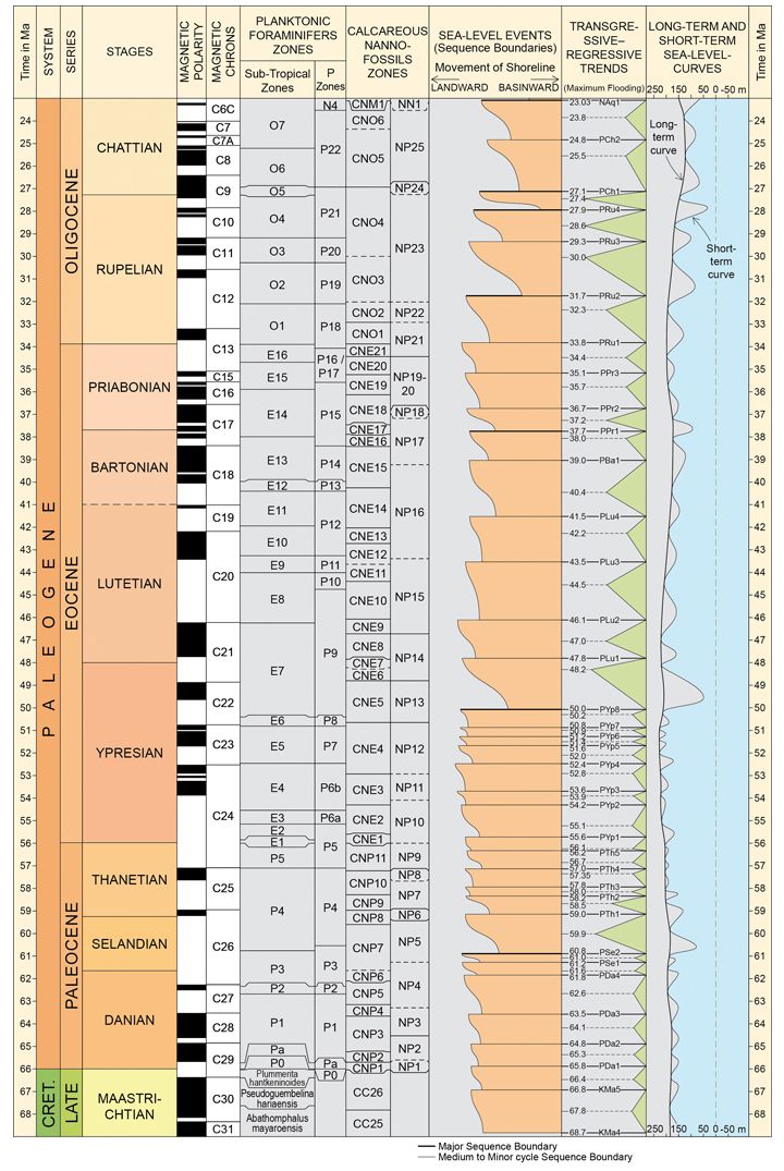
Paleogene depositional sequences and eustatic sea-level variations. Numerical time scale, magnetostratigraphy, and biostratigraphic zones after various authors (in Gradstein et al., 2020). Sequence boundaries are labeled with unique alphanumeric designations (third column from right), where first letter “P” is for Paleogene, followed by two first letters of the Stage name and a number to identify the oldest to youngest events in that Stage. Also listed in this column are the ages of the sequence boundaries and maximum flooding surfaces that have been calibrated to δ18O data (after Westerhold et al., 2020).

Figure 2

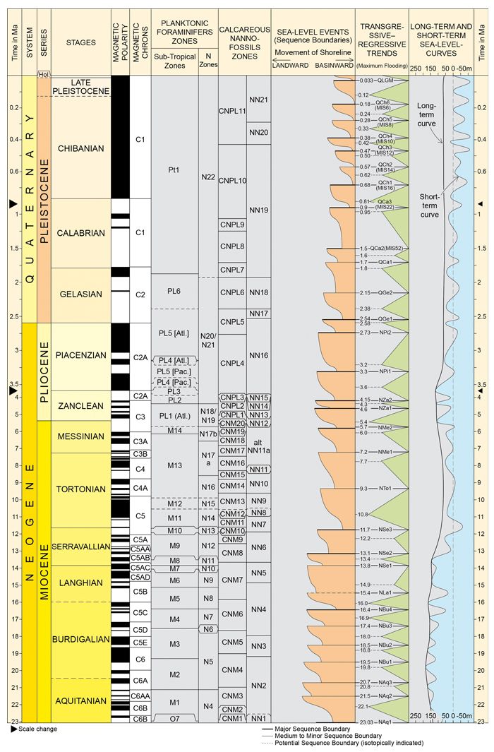
Neogene and Quaternary depositional sequences and eustatic sea-level variations. Numerical time scale, magnetostratigraphy, and biostratigraphic zones after various authors (in Gradstein et al., 2020). Sequence boundaries are labeled with unique alphanumeric designations (third column from right), where first letter “N” and “Q” stand for Neogene and Quaternary, respectively, followed by two first letters of the Stage name and a number to identify the oldest to youngest events in that Stage. Also listed in this column, the ages of sequence boundaries (SB) and maximum flooding surfaces that have been fine-tuned by calibrations with oxygen-isotopic data. For the Quaternary sequences 1.5 Ma and younger, Marine Isotope Stage numbers (e.g., MIS22) in which the SB occurs are also added. The youngest SB that was caused by the withdrawal of the sea during the Last Glacial Maximum is designated as QLGM. [Note: the scale changes at 3.6 and 1.8 Ma in the numerical time scale columns.]

The Cenozoic eustatic framework presented here reconciles more recent sequence-stratigraphic documentation and ties the SL curves to the latest versions of the biochronologic time scale. We have discussed our rationale for refining the ages of the third order as well as higher-frequency sequence boundaries and MFSs through δ¹⁸O calibrations. We have also discussed our reasons for not professing purely quantitative estimates of the amplitude of SL changes, as both the stratigraphic and isotopic estimates incorporate numerous critical sources of uncertainty in calculating these values. In a best-case scenario, benthic δ¹⁸O_sw aided by Mg/Ca ratios could yield such desirable quantitative measures, at least since the onset of major ice sheets on land. Nevertheless, in practice the realty is different; studies that have relied on isotopic data alone to produce amplitude estimates, where there are many uncertainties, are no more accurate than those relying on stratigraphic data alone, where local factors can bias our calculations. In the current revision, for the pre-Quaternary, we continue to rely of the global averaging approach, aided by isotopic data where possible, to get an improved sense of the global mean from several noncontiguous locations. We have to face the fact that meaningful precision with respect to amplitude is not attainable with the methodologies available and we can only guesstimate the eustatic ups and downs using multiple criteria.

Finally, because most Cenozoic fine-tuned, third-order sequence durations fall within the range of long-period modulations of the obliquity (1.2 m.y.) and eccentricity (2.4 m.y.), it is reasonable to affirm that third-order depositional cycles have a close link to major climatic variations, with deviations caused by the tectonic overprint (see further discussion in the Supplemental Material).

The authors would like to acknowledge the reviewers who pointed to important additional documentation and helped improve the text. The figures were drafted at Sorbonne University, Institute of Earth Sciences, by Alexandre Lethiers, whose diligence is duly acknowledged.

1. Adkins, J.F., McIntyre, K., and Schrag, D.P., 2002, The salinity, temperature and δ¹⁸O of the glacial deep ocean: Science, v. 298, no. 5599, p. 1769–1773, https://doi.org/10.1126/science.1076252.
2. Boulila, S., Peters, S.E., Müller, R.D., Haq, B.U., and Hara, N., 2023, Earth’s interior dynamics drive marine fossil diversity cycles of tens of millions of years: Proceedings of the National Academy of Sciences of the United States of America, v. 120, no. 29, https://doi​.org/10.1073/pnas.2221149120.
3. Cloetingh, S., McQueen, H., and Lambeck, K., 1985, On a tectonic mechanism for regional sea-level variations: Earth and Planetary Science Letters, v. 75, no. 2–3, p. 157–166, https://doi.org/10.1016/​0012-821X(85)90098-6.
4. Cloetingh, S., and Haq, B.U., 2015, Inherited landscapes and sea-level change: Science, v. 347, no. 6220, https://doi.org/10.1126/science.1258375.
5. Cramer, B.S., Toggweiler, J.R., Wright, J.D., Katz, M.E., and Miller, K.G., 2009, Ocean overturning since the Late Cretaceous: Inferences from a new benthic foraminiferal isotope compilation: Paleoceanography, v. 24, no. 4, https://doi.org/10.1029/​2008PA001683.
6. Davies, D.R., Ghelichkhan, S., Hoggard, M., Valentine, A.P., and Richards, F.D., 2023, Observations and models of dynamic topography: Current status and future directions, in Duarte, J., ed., Dynamics of Plate Tectonics and Mantle Convection: Amsterdam, Elsevier, p. 223–269, https://doi.org/10.1016/B978-0-323-85733-8.00017-2.
7. Dawber, C.F., and Tripati, A.K., 2011, Constraints on glaciation in the middle Eocene (46–37 Ma) from Ocean Drilling Program, Site 1209 in the tropical Pacific Ocean: Paleoceanography, v. 26, no. 2, https://doi.org/10.1029/2010PA002037.
8. DeConto, R.M., and Pollard, D., 2003, Rapid Cenozoic glaciation of Antarctica induced by declining atmospheric CO₂: Nature, v. 421, no. 6920, p. 245–249, https://doi.org/10.1038/nature01290.
9. Elderfield, H., Ferretti, P., Greaves, M., Crowhurst, S., McCave, I.N., and Piotrowski, A.M., 2012, Evolution of the ocean temperature and ice volume through the Mid-Pleistocene Climate Transition: Science, v. 337, no. 6095, p. 704–709, https://doi.org/10.1126/science.1221294.
10. Gibbard, P.L., and Head, M.J., 2020, The Quaternary Period, in Gradstein F.M., Ogg, J.G., Schmitz, M.D., and Ogg, G.M, eds., The Geological Time Scale 2020, v. 2: Amsterdam: Elsevier, p. 1217–1255, https://doi.org/10.1016/B978-0-12-824360-2.00030-9.
11. Gradstein, F.M., Ogg, J.G., Schmitz, M.D., and Ogg, G.M., eds., 2020, The Geological Time Scale 2020, .] 2: Amsterdam, Elsevier, 1390 p.
12. Haq, B.U., 2014, Cretaceous eustasy revisited: Global and Planetary Change, v. 113, p. 44–58, https://doi.org/10.1016/j.gloplacha​.2013.12.007.
13. Haq, B.U., 2018a, Jurassic sea-level variations: A reappraisal: GSA Today, v. 28, no. 1, p. 4–10, https://doi.org/10.1130/GSATG359A.1.
14. Haq, B.U., 2018b, Triassic eustatic variations reexamined: GSA Today, v. 28, no. 12, p. 4–9, https://doi.org/10.1130/GSATG381A.1.
15. Haq, B.U., and Al-Qahtani, A.M., 2005, Phanerozoic cycles of sea-level change on the Arabian Platform: GeoArabia, v. 10, p. 127–160, https://doi.org/10.2113/geoarabia1002127.
16. Haq, B.U., and Schutter, S.R., 2008, A chronology of Paleozoic sea-level changes: Science, v. 322, p. 64–68, https://doi.org/10.1126/science.1161648.
17. Haq, B.U., Hardenbol, J., and Vail, P.R., 1987, Chronology of fluctuating sea levels since the Triassic: Science, v. 235, no. 4793, p. 1156–1167, https://doi.org/10.1126/science.235.4793.1156.
18. Haq, B.U., et al., 1988, Mesozoic and Cenozoic chronostratigraphy and cycles of sea-level change, in Wilgus, C.K., Hastings, B.S., Posamentier, H., Van Wagoner, J., Ross, C.A., and Kendall, C.G., eds., Sea-Level Changes: An Integrated Approach: SEPM Special Publication, v. 42, p. 71–108, https://doi.org/10.2110/pec.88.01.0071.
19. Hardenbol, J., Thierry, J., Farley, M.B., Jacquin, T., de Graciansky, P.-C., and Vail, P.R., 1998, Mesozoic and Cenozoic sequence chronostratigraphic framework of European basins, in de Graciansky, P.-C., Hardenbol, J., Thierry, J., and Vail, P.R., eds., Mesozoic and Cenozoic Sequence Stratigraphy of European Basins: SEPM Special Publication, v. 60, p. 3–13.
20. Horita, J., Zimmermann, H., and Holland, H.D., 2002, Chemical evolution of seawater during the Phanerozoic: Implications from the record of marine evaporites: Geochimica et Cosmochimica Acta, v. 66, no. 21, p. 3733–3756, https://doi.org/10.1016/S0016-7037(01)00884-5.
21. Kominz, M.A., Browning, J.V., Miller, K.G., Sugarman, P.J., Mizintseva, S., and Scotese, C.R., 2008, Late Cretaceous to Miocene sea level estimates from New Jersey and Delaware coastal plain coreholes: Basin Research, v. 20, no. 2, p. 211–226, https://doi.org/10.1111/​j.1365-2117.2008.00354.x.
22. Kominz, M.A., Miller, K.G., Browning, J.V., Katz, M.E., and Mountain, G.S., 2016, Miocene relative sea level on the New Jersey shallow continental shelf and coastal plain derived from one-dimensional backstripping: A case for both eustasy and epeirogeny: Geosphere, v. 12, no. 5, p. 1437–1456, https://doi.org/10.1130/GES01241.1.
23. Lear, C.H., Bailey, T.R., Pearson, P.N., Coxall, H.K., and Rosenthal, Y., 2008, Cooling and ice growth across the Eocene-Oligocene transition: Geology, v. 36, no. 3, p. 251–254, https://doi.org/10.1130/G24584A.1.
24. Miller, K.G., Mountain, G.S., Browning, J.V., Kominz, M., Sugarman, P.J., Christie-Blick, N., Katz, M.E., and Wright, J.D., 1998, Cenozoic global sea level, sequences, and the New Jersey Transect: Results from coastal plain and slope drilling: Reviews of Geophysics, v. 36, no. 4, p. 569–601, https://doi.org/10.1029/98RG01624.
25. Miller, K.G., Wright, J.D., Katz, M.E., Browning, J.V., Cramer, B.S., Wade, B.S., and Mizintseva, S.F., 2008, A view of Antarctic ice-sheet evolution from sea level and deep-sea isotope changes during the Late Cretaceous–Cenozoic, in Cooper, A.K., et al., eds., Antarctica: A Keystone in a Changing World: Proceedings of the 10th International Symposium on Antarctic Earth Sciences: Washington, D.C., National Academies Press, p. 55–70.
26. Miller, K.G., Browning, J.V., Schmelz, W.J., Kopp, R.E., Mountain, G.S., and Wright, J.D., 2020, Cenozoic sea level and cryospheric evolution from deep-sea geochemical and continental margin records: Science Advances, v. 6, no. 20, https://doi.org/10.1126/sciadv.aaz1346.
27. Moucha, R., Forte, A.M., Mitrovica, J.X., et al., 2008, Dynamic topography and long-term sea-level variations: There is no such thing as a stable continental platform: Earth and Planetary Science Letters, v. 271, p. 101–108, https://doi.org/10.1016/j.epsl.2008.03.056.
28. Müller, R.D., Sdrolias, M., Gaina, C., Steinberger, B., and Heine, C., 2008, Long-term sea-level fluctuations driven by ocean basin dynamics: Science, v. 319, p. 1357–1362, https://doi.org/10.1126/science.1151540.
29. Müller, R.D., Hassan, R., Gurnis, M., Flament, N., and Williams, S.E., 2018, Dynamic topography of passive continental margins and their hinterlands since the Cretaceous: Gondwana Research, v. 53, p. 225–251, https://doi.org/10.1016/j.gr.2017.04.028.
30. Pearson, P.N., 2012, Oxygen isotopes in foraminifera: Overview and historical review: The Paleontological Society Papers, v. 18, p. 1–38, https://doi.org/10.1017/S1089332600002539.
31. Raffi, I., et al., 2020, The Neogene Period, in Gradstein F.M., Ogg, J.G., Schmitz, M.D., and Ogg, G.M, eds., The Geological Time Scale 2020, v. 2: Amsterdam, Elsevier, p. 1141–1215, https://doi.org/10.1016/B978-0-12-824360-2.00029-2.
32. Raymo, M.E., Kozdon, R., Evans, D., Lisiecki, L., and Ford, H.L., 2018, The accuracy of mid-Pliocene δ¹⁸O-based ice volume and sea level reconstructions: Earth-Science Reviews, v. 177, p. 291–302, https://doi.org/10.1016/j.earscirev.2017.11.022.
33. Rowley, D.B., Forte, A.M., Moucha, R., Mitrovica, J.X., Simmons, N.A., and Grand, S.P., 2013, Dynamic topography change of the eastern United States since 3 million years ago: Science, v. 340, p. 1560–1563, https://doi.org/10.1126/science.1229180.
34. Schmelz, W.J., Miller, K.G., Kopp, R.E., Mountain, G.S., and Browning, J.V., 2021, Influence of mantle dynamic topographical variations on US Mid‐Atlantic margin estimates of sea‐level change: Geophysical Research Letters, v. 48, no. 4, https://doi.org/10.1029/2020GL090521.
35. Spasojević, S., Liu, L., Gurnis, M., and Müller, R.D., 2008, The case for dynamic subsidence of the United States East Coast since the Eocene: Geophysical Research Letters, v. 35, no. 8, https://doi.org/​10.1029/2008GL033511.
36. Speijer, R.P., Pälike, H., Hollis, C.J., Hooker, J.J., and Ogg, J.G., 2020, The Paleogene Period, in Gradstein F.M., Ogg, J.G., Schmitz, M.D., and Ogg, G.M., eds., The Geological Time Scale 2020, v. 2: Amsterdam, Elsevier, p. 1087–1140, https://doi.org/10.1016/B978-0-12-824360-2.00028-0.
37. Valdes, P.J., Scotese, C.R., and Lunt, D.J., 2021, Deep ocean temperatures through time: Climate of the Past, v. 17, p. 1483–1506, https://doi.org/10.5194/cp-17-1483-2021.
38. Westerhold, T., et al., 2020, An astronomically dated record of Earth’s climate and its predictability over the last 66 million years: Science, v. 369, no. 6509, p. 1383–1387, https://doi.org/10.1126/science.aba6853.