Google Earth Engine Web Applications for Investigating and Teaching Fundamental Geoscience Concepts

Andrew K.R. Hoxey

University of Kansas, Department of Geology, Lawrence, Kansas 66045, USA

Michael H. Taylor

University of Kansas, Department of Geology, Lawrence, Kansas 66045, USA

J. Douglas Walker

University of Kansas, Department of Geology, Lawrence, Kansas 66045, USA

Diane L. Kamola

University of Kansas, Department of Geology, Lawrence, Kansas 66045, USA

Cloud computing that queries public data enables rapid geographic information system analysis, reducing the processing time required for complex raster calculations on remote sensing data. When combined with cloud computing, web applications allow users with no experience in computing languages to access computing power as long as users have an internet connection, whether in the classroom, the field, or a research lab. We present two web applications developed on the Google Earth Engine platform that enable topographic and structural analyses on remote sensing data through a graphical user interface, expanding the accessibility of earth sciences.

The Google Earth Engine Plane Orientation Calculator web application calculates an orientation (strike and dip) of the plane defined by three user-selected points on a digital elevation model. The tool utilizes established methods of interpreting map patterns and elevations (i.e., the three-point problem) to understand the geometry of surface features, a fundamental interest to structural geologists and geologic studies. The Plane Orientation Calculator combines fundamental geologic mapping concepts and cloud computing web application to make it possible to measure structural features at any location on Earth within the coverage of public data. Users can make multiple measurements, catalog locations and orientations, and export data for use in other software. The simplicity of the tool means users at all experience levels can conduct remote geologic mapping.

Topographic swath profiles display elevation data, local relief, and regional trends in topography—an approach that is commonly used to identify areas of interest to geologists and geomorphologists. The Google Earth Engine Topographic Swath Profiler web application rapidly queries public digital elevation models selected by the user to produce topographic swath profiles. Users can customize the swath length, swath width, and sampling rate before displaying or exporting the sampled data as text or vector files. Topographic swath profiles are generated instantly via cloud computing, reducing the investment of time and computing budget typically required for such analysis.

*andrew.hoxey@ku.edu
CITATION: Hoxey, A.K.R., Taylor, M.H., Walker, J.D., and Kamola, D.L., 2024, Google Earth Engine web applications for investigating and teaching fundamental geoscience concepts: GSA Today, v. 34, p. 4–10, https://doi.org/10.1130/GSATG588A.1.
© 2024 The Authors. Gold Open Access: This paper is published under the terms of the CC-BY-NC license. Printed in USA.
Manuscript received 8 October 2023. Revised manuscript received 6 February 2024. Manuscript accepted 30 April 2024. Posted 4 June 2024.

Physical and financial barriers to field investigations hinder retention in undergraduate programs (Hall et al., 2004; Giles et al., 2020) and have led to historical shortcomings in diversity, equity, and inclusion within the geoscience community (Núñez et al., 2020; Posselt and Nuñez, 2022). In response, several initiatives are focused on increasing accessibility and encouraging the development of virtual tools that supplement field experiences and expand accessibility (National Academies of Sciences, Engineering, and Medicine, 2020; Bursztyn et al., 2022; Pugsley et al., 2021). Similarly, cloud computing for GIS data processing has expanded the capabilities of researchers, industry professionals, and educators working with large data sets (Gorelick et al., 2017; Bhat et al., 2011; Krishnan et al., 2011).

Here we describe two Google Earth Engine (GEE) web applications (Gorelick et al., 2017)—the Plane Orientation Calculator (POC; andrewhoxey.com/online-tools/poc) and the Topographic Swath Profiler (TSP; andrewhoxey.com/online-tools/tsp)—designed for novice to expert users to interrogate global digital elevation models (DEMs). Web applications combine the speed and power of cloud computing with a graphical user interface (GUI) that can be operated with a mobile device from anywhere with internet access.

Surface orientations are fundamental for geologic and structural maps and can inform interpretations of subsurface geometries, fault kinematics, and slope stability. The POC makes gathering surface geometry data possible anywhere within the coverage of the GEE DEM catalog (Fig. 1). Similar tools are commonly used for remote and reconnaissance mapping (Alberti, 2019; Allmendinger, 2020) but typically require expertise with GIS software to aggregate, process, and store data. The POC, by contrast, is optimized to make start-up simple and rapid.

Figure 1

The Plane Orientation Calculator (POC) calculates the orientation of a plane from user-selected points. Once users have identified three points (dark blue) that are representative of a plane, an orientation is calculated and displayed in the results panel. Saved points (light blue dots) are plotted and available to export as a .csv file.

The Plane Orientation Calculator (POC) calculates the orientation of a plane from user-selected points. Once users have identified three points (dark blue) that are representative of a plane, an orientation is calculated and displayed in the results panel. Saved points (light blue dots) are plotted and available to export as a .csv file.

The first step in using the POC is considering the scale of the feature being measured, the ability to accurately place points, and the resolution of the data being queried (Fig. 1). After navigating to an area of interest, users can select from various data catalogs, including high-resolution (e.g., USGS 3DEP 1 m) DEMs where available (U.S. Geological Survey, 2019). The “DEM in Use” drop-down menu includes eight options that will generate new layers of a local hillshade, contours, and an elevation color scale visible in the layers palette after clicking “RESET LOCAL DEM.” Making the contour layer visible can be computationally intensive, but reducing the range of elevations covered by the contours and adjusting the contour interval can reduce computation time significantly. Once a local DEM is selected, the “Extent of Selected DEM” layer will also appear in the layer palette and show the spatial coverage of the catalog. The “RESET LOCAL DEM” button should be clicked after panning to a new region.

A crosshair cursor in the map viewer indicates when users can select a point. Points may be selected along geologic contacts, for example, a fault that Vs into a valley, or on a dip-slope. Users should consider all the data available, make an interpretation of the geology, and carefully place points to characterize the plane of interest. Closely spaced contours that overlay the imagery are particularly helpful for placing points accurately. After three points are created, the user can edit points by clicking and dragging their associated balloons. Once the user is satisfied with the point placement, clicking “CALCULATE” will yield an orientation of the plane defined by the three points.

After the calculation yields a result, users can elect to save the result, make edits to existing points, or discard the result. When a calculated orientation is saved, the result is recorded as a new feature at the location of the highest-elevation point. Multiple calculation results can be recorded in the saved points panel, will be added to the map as a new layer, and can be exported as a .csv file that includes location and orientation data.

The orientation is calculated by (1) querying the DEM for values, (2) evaluating the relationship between the points as vectors, and (3) using the vectors to determine the orientation of the plane.

Querying the DEM employs the native GEE reducer function (ee.Image.reduceRegions()) and yields the elevation value of the nearest cell centroid. Changes in the zoom level will update the map display and resample the DEM, but data catalogs are queried at their native resolution, not the active pyramid level. Querying the DEM’s native resolution may cause unexpected results relative to the map viewer but will reduce uncertainty when used properly.

The distances between user-selected points are calculated in the x, y, and z directions. Determining the x and y distances independently using the native GEE function (ee.Feature.distance()) requires the formation of a third (t) point at the intersection of the two points’ latitude and longitude, respectively. For example, the ee.Feature.distance() function for the high-elevation (h) and low-elevation (l) points returns the hypotenuse of a right triangle defined by the three points (h, l, t) in x–y space. Rather than applying trigonometry with a bearing between the two points (h, l), our approach of creating a third point and a right triangle minimizes the computational budget. All distances (x, y, z) are calculated relative to the highest-elevation (h) point such that the middle-elevation (m) and low-elevation (l) points can be characterized by vectors [xh-m, yh-m, zh-m] and
[xh-l, yh-l, zh-l], where negative values in x and y correlate to west and south, respectively.

Vector multiplication is a simple computation in most software and is commonly employed for calculating plane orientations (Vacher, 2000). Following the procedures of Vacher (2000), the POC script uses the native GEE function (ee.Array.matrixSolve()) to determine the slope of the plane in the x and y directions, then convert the result to strike and dip using trigonometry.

Data analysis using GEE has varying degrees of uncertainty that are dependent on the data set being queried, the zoom level, and the accuracy of the user selection. When selecting an area of interest, users should consider the measured feature’s scale, the ability to accurately place points, the alignment of satellite imagery with elevation data, and the resolution of the DEM. Different data catalogs within GEE have varying measures of uncertainties by nature of the publisher’s processing method and the reprojection in GEE. Rather than considering the precision of each catalog independently and propagating values through the calculation, we take a simplified approach by creating subparallel planes generated using the variance in the elevation within a nine-cell region around the queried points (Fig. 2A).

Figure 2

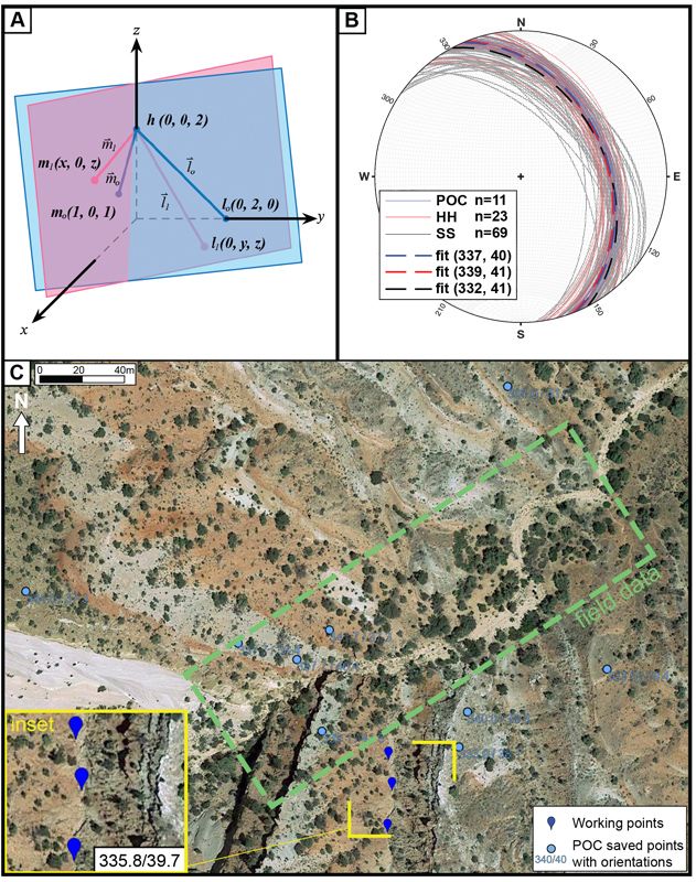
(A) Schematic diagram describing the framework for the uncertainty calculation. Translating the low-elevation point (l) and mid-elevation point (m) away from the original plane (blue) by a distance equal to the measured uncertainty yields a new plane (red) with an orientation that characterizes the precision. (B) Stereonet including all the data collected using the Plane Orientation Calculator (POC; blue planes), hand-held compass measurement (HH; red planes), and StraboSpot2 software (SS; black planes). Online data was collected using USGS 3DEP 1-m DEM (U.S. Geological Survey, 2019). (C) Screenshot from POC showing the area where data was collected in southwest Utah. Blue dots show the location of POC measurements. The green box shows the location of field measurements. The inset map shows the three points (blue) selected along a lithologic contact for measurement #11 and the yielded orientation (see Supplemental Material [see footnote 1]). POC-queried features include other lithologic boundaries, dip-slopes, and laterally continuous beds that V across the gulch.

(A) Schematic diagram describing the framework for the uncertainty calculation. Translating the low-elevation point (l) and mid-elevation point (m) away from the original plane (blue) by a distance equal to the measured uncertainty yields a new plane (red) with an orientation that characterizes the precision. (B) Stereonet including all the data collected using the Plane Orientation Calculator (POC; blue planes), hand-held compass measurement (HH; red planes), and StraboSpot2 software (SS; black planes). Online data was collected using USGS 3DEP 1-m DEM (U.S. Geological Survey, 2019). (C) Screenshot from POC showing the area where data was collected in southwest Utah. Blue dots show the location of POC measurements. The green box shows the location of field measurements. The inset map shows the three points (blue) selected along a lithologic contact for measurement #11 and the yielded orientation (see Supplemental Material [see footnote 1]). POC-queried features include other lithologic boundaries, dip-slopes, and laterally continuous beds that V across the gulch.

For example, the [x, y, z] describes the position of the low-elevation point (l) relative to the high-elevation point (h). For elevation, the standard deviation of the nine-cell neighborhood determines zmax and zmin (Fig. 2A). For the x and y values, the native GEE function (ee.Feature.distance()) has some inherent uncertainty that is dependent on the projection of the DEM. Since all projections will have different results and we want the tool to remain as universal as possible, we impose a 5% uncertainty to all distance calculations. The six values ([xmin, ymin, zmin] and [xmax, ymax, zmax]) effectively buffer the point in 3-D space.

The geometry of a plane dictates that substituting the minimum x, y, and z values of the vector results in a translation along the original plane. By contrast, the maximum x, y, and minimum z values result in a new point that is translated away from the original plane. For the uncertainty calculation, we consider the values that generate two new points (m1, l1) translated away from the original plane (Fig. 2A). Holding the high-elevation point (h) constant and calculating the orientation of the plane defined by (h, m1, l1) results in a new strike and dip. We calculate two different planes: (1) translating point m0 up and away while translating point l0 down and toward point h (h, m1, l1), and (2) translating point m0 down and toward while translating point l0 up and away from point h (h, m2, l2). The resulting planes represent the maximum rotation within the bounds of the queried values ([xmin, ymin, zmin] and [xmax, ymax, zmax]) and yield new strikemin,max and dipmin,max values displayed in the results panel.

In contrast to considering each DEM’s projection and uncertainty independently, the method of deriving subparallel planes has the benefit of being simple and universal. While a more statistical approach that considers the quality of each DEM may result in greater confidence, the simplicity of the computation keeps the tool functional. The largest uncertainties in elevation are typically yielded when the neighborhood surrounding the selected points has a high variance (i.e., high local relief). For example, cliff faces generally yield elevation values with low precision relative to low-slope, laterally extensive surfaces, so users should consider the relief within the neighborhood of each selected point and avoid local topographic anomalies. Regardless of the DEM’s resolution, large uncertainties are also yielded when the three points selected are separated by large distances in the x and y directions. The map distance is always assigned 5% uncertainty, even when selecting points that are separated by hundreds of kilometers, meaning closely spaced points yield more precise results.

Reconnaissance mapping using remote sensing data is an important component of field research, particularly in remote and inaccessible areas where mapping is often supplemented by interpretations of imagery (e.g., DeCelles et al., 2020; Baltz et al., 2021). Similarly, accessibility problems with undergraduate field mapping courses or inclement weather can hinder data collection during student exercises. To test the viability of using the POC as a method of geologic mapping, here we compare data collected in the field using hand-held compasses, a tablet equipped with the StraboSpot2 geologic data collections app (Walker et al., 2019), and the POC (Figs. 2B and 2C).

Outcrops of Jurassic sedimentary rocks in the southeast portion of Capitol Reef National Park provide an ideal laboratory because the rocks are well exposed, it is within the coverage of the USGS 1 m elevation data, and beds are consistently northeast-dipping (Figs. 2B and 2C; Hintze and Stokes, 1963; U.S. Geological Survey, 2019). Data were queried using the POC by placing points at 5–10 m spacing on continuous surfaces or along geologic contacts identified using the hillshade, contours, and satellite imagery (Fig. 2C inset; Supplemental Material1). In the field, data was collected using the StraboSpot2 app on an 11-inch iPad and by undergraduate students using standard Brunton compasses to simulate results of a student exercise (see Supplemental Material). Results are similar within typical variation, indicating the POC yields results that are a close approximation of the geology and a classroom setting. Our results indicate that the POC is a reliable virtual substitute for field measurements when bedrock orientations are well expressed in the DEM. Furthermore, the compatibility of the POC with mobile devices makes impromptu data collection possible, increasing the accessibility of geologic investigation.

-------
1Supplemental Material. Table of measurements used in Plane Orientation Calculator example. Please visit https://doi.org/10.1130/GSAT.S.25878097 to access the supplemental material, and contact editing@geosociety.org with any questions. All scripts are available at https://github.com/andrewkrh/GEE_GeologyTools.

Topographic swath profiles can be broadly described as a series of parallel cross-sectional topographic profiles sampled within a region and projected onto a single plane. They are commonly used by geoscientists to describe the first-order topographic expression of geologic phenomena, such as mountain belts (Burbank et al., 2003; Bookhagen and Burbank, 2006). The Topographic Swath Profiler (TSP) is a web application that allows users to conduct rapid topographic analysis with little time investment or coding expertise (Fig. 3).

Figure 3

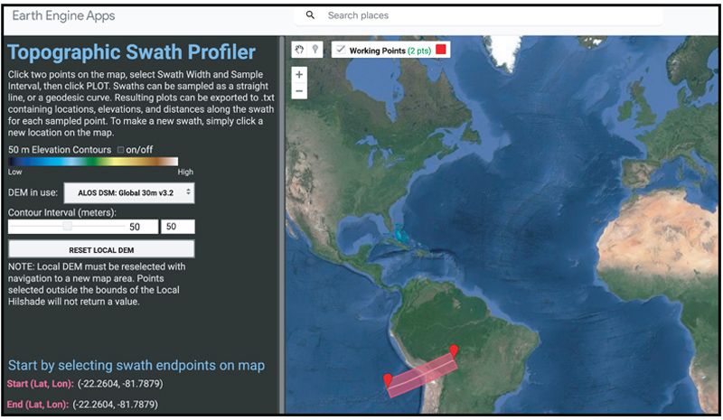
A screenshot from the Topographic Swath Profiler (TSP) shows an example swath location. The TSP allows users to generate continental-scale topographic swath profiles instantly.

A screenshot from the Topographic Swath Profiler (TSP) shows an example swath location. The TSP allows users to generate continental-scale topographic swath profiles instantly.

The TSP allows users to select from multiple DEMs of varying resolutions. Choosing an ideal DEM resolution is an important step in topographic analysis regardless of the processing interface. Users should consider the scale of the features being investigated and the importance of resolving any detail within the feature. By default, the TSP is designed to sample the selected DEM at its native resolution, regardless of the pyramid level displayed in the map viewer, which may include cell resampling. As a result, anomalies in high-resolution data that may not be visible in the map viewer will be included in the output profile, and attention should be paid to the selection of the DEM and how it is displayed. On selecting a DEM, the user must click “RESET LOCAL DEM” to generate new layers in the layer palette.

Once the appropriate data set is selected, clicking the map area will create start and end points for the desired swath. A polygon outlining the sampling region will automatically generate and refresh with changes to the dimensions. The start and end points can be edited by clicking on the balloons and moving them as needed, and two sliders control the swath width and sampling rate. Swath width is measured as a fraction of the length and can be adjusted to as large as 50% (1:2 aspect ratio), while sample density is measured as a percent of the selected DEM’s native resolution. As discussed in a later section, the TSP is limited to processing no more than 20,000 data points, so larger swaths may require a reduction in the sample density.

Once the swath profile dimensions are set, clicking “PLOT” generates two distance-versus-elevation plots visible in the results panel. The top panel includes all the points sampled, and the bottom panel is a line plot showing minimum, maximum, and mean elevations with distance along the swath. The plots can be exported from GEE as .svg files, or users can export the results as a .csv file. Note that the charts displayed do not feature consistent aspect ratios, meaning the vertical exaggeration will vary, and advanced users may prefer to export data for use in other plotting software. Exported KML files will include the line between the selected points and a polygon of the swath bounds.

The primary advantage of the TSP is the speed and accessibility of GEE web applications that make it possible to rapidly investigate areas of interest globally. However, limitations of processing capacity and data reprojections may make the TSP undesirable for research applications in comparison to other methods of generating topographic swath profiles (Schwanghart and Scherler, 2014; Forte and Whipple, 2019).

In contrast to other topographic analysis tools that are limited only by the user’s local processing capacity, GEE limits the processing quota to 10 MB per query, which equates to ~20,000 data points in a swath, meaning resampling is often necessary. Resampling is executed via raster scaling, meaning rasters are resampled to a user-defined scale prior to being queried. The resampling slider is designed to be intuitive for beginners and is measured as a percent of the DEM’s original resolution, where a lower percent equates to a lower sampling rate. For example, using a 30-m-resolution DEM and a 50% sample density will result in a 60-m-resolution DEM where all the 60 m cells are included in the swath profile. Advanced users should consider the GEE scaling limitations and the resampling method when selecting from the available DEMs, as resampling high-resolution DEMs may introduce large uncertainty.

Global projections can also lead to unexpected results when data are projected to the swath. Reprojecting images in the GEE interface is discouraged even when working with varying data sets. As a result, calculating a cell’s along-swath distance (distX) is simplified by calculating the length of the center line with ee.Geometry.length() and dividing by the sample density. A series of swath-perpendicular lines yields columns of values queried from cells that intersect a given line. All values in a column are assigned the same along-swath distance (distX) regardless of the queried cell’s centroid location or the distance from the swath’s center line (distY). The global projection and distance calculation ignores differences in lengths between the upper and lower bounds of a swath, potentially yielding inconsistencies in regional-scale (>1000 km length) or cross-polar swaths.

The limitations of processing capacity and reprojections are a necessary trade-off for global usability and accessibility. The benefits outweigh the negatives for most instances of reconnaissance investigation or student engagement.

Using the TSP in undergraduate courses allows students to engage with fundamental relationships between geologic processes and topography by querying research-grade data. For example, users can describe the geometric variations in subduction zones by generating topographic swath profiles across convergent margins (Figs. 4A–4C). Three swaths generated with the TSP across the Altiplano, Cascadia, and Japan clearly illustrate how subduction interfaces with differing ages and compositions of the crust result in different topographic and bathymetric signatures. Similar results can be generated with an elevation profile in Google Earth Pro, which samples elevations along a single line of low-resolution data. Generating a topographic swath smooths anomalous noise and facilitates greater discussion on local relief or the potential for along-strike variation. In any classroom where students have access to the internet, high-resolution DEMs can be used for introducing students to concepts like the angle of repose on sand dunes or the formation of marine terraces.

Figure 4

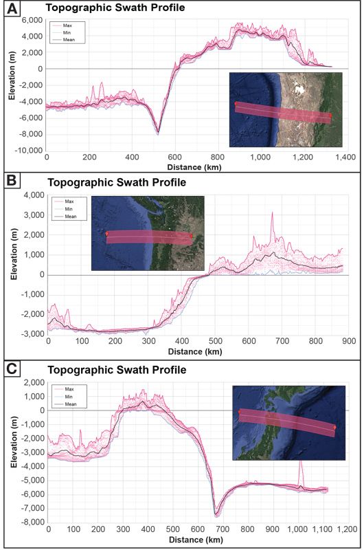
Example of classroom use for the Topographic Swath Profiler (TSP). Data were sampled across three sites: Altiplano, Cascadia, and Japan (A–C, respectively). Because the TSP is simple and fast, novice users can compare features in minutes. Elevation data from ALOS 30 m global (Takaku et al., 2020).

Example of classroom use for the Topographic Swath Profiler (TSP). Data were sampled across three sites: Altiplano, Cascadia, and Japan (A–C, respectively). Because the TSP is simple and fast, novice users can compare features in minutes. Elevation data from ALOS 30 m global (Takaku et al., 2020).

The TSP is also a powerful reconnaissance and hypothesis-building tool for researchers investigating new regions. Available tools for generating topographic swath profiles often require reprojecting and resampling DEMs (Schwanghart and Scherler, 2014), which can be nontrivial depending on the user’s experience level and the data availability, implying a time investment. Cloud computing eliminates the preparation process and makes analysis possible with a mobile device, supplementing investigations and inspiring new questions in the office or in the field.

The availability of cloud computing and public data catalogs is increasing the accessibility of analysis, allowing for creative and innovative ways to engage with earth sciences. We present two web applications developed on the GEE online interface that can be used by workers with no computational background to query DEMs. The Plane Orientation Calculator (POC) and Topographic Swath Profiler (TSP) query global data sets, are accessible to anyone with an internet connection, and are designed to be user-friendly and rapid.

The POC uses fundamental geometric principles to calculate the orientations of planes defined by user-selected points on the surface of the Earth. The web application combines the accessibility of data in GEE with a proven method for calculating structural orientations into a tool for reconnaissance mapping, remote data collection, and student engagement. The TSP is similarly designed for rapid computing and ease of use in querying DEMs to produce topographic swath profiles. Topographic swath profiles are a commonly employed representation of the topographic expression of geologic phenomena. However, constructing topographic swath profiles typically requires nontrivial background knowledge and GIS software that creates an obstacle for users with limited time or experience. With the TSP, novice users can interrogate global data sets and produce topographic swath profiles. The tools described above increase the accessibility of data collection and topographic analysis to any user with a mobile device connected to the internet, making them useful tools for research, virtual field trips, and introducing geologic concepts in classroom settings.

We thank the students of the University of Kansas field camp who collected hand-held compass data. Clay Campbell, Dan Mongovin, and Hillary Mwongyera helped with beta testing. This manuscript was greatly improved by reviews from two anonymous reviewers.

1. Alberti, M., 2019, GIS analysis of geological surfaces orientations: The qgSurf plugin for QGIS: PeerJ Preprints, v. 7, https://doi.org/10.7287/peerj.preprints.27694v1.
2. Allmendinger, R.W., 2020, GMDE: Extracting quantitative information from geologic maps: Geosphere, v. 16, p. 1495–1507, https://doi.org/​10.1130/GES02253.1.
3. Baltz, T., Murphy, M., Fan, S., and Chamlagain, D., 2021, Geometry, kinematics, and magnitude of extension across the Thakkhola Graben, Central Nepal Himalaya: Journal of Nepal Geological Society, v. 62, p. 1–17, https://doi.org/10.3126/jngs.v62i0.38691.
4. Bhat, M.A., Shah, R.M., and Ahmad, B., 2011, Cloud computing: A solution to geographical information systems (GIS): International Journal of Advanced Trends in Computer Science and Engineering, v. 3, no. 2, p. 594–600.
5. Bookhagen, B., and Burbank, D.W., 2006, Topography, relief, and TRMM‐derived rainfall variations along the Himalaya: Geophysical Research Letters, v. 33, p. 1–5, https://doi.org/10.1029/2006GL026037.
6. Burbank, D.W., Blythe, A.E., Putkonen, J., Pratt-Sitaula, B., Gabet, E., Oskin, M., Barros, A., and Ojha, T.P., 2003, Decoupling of erosion and precipitation in the Himalayas: Nature, v. 426, p. 652–655, https://doi.org/10.1038/nature02187.
7. Bursztyn, N., Sajjadi, P., Riegel, H., Huang, J., Wallgrün, J.O., Zhao, J., Masters, B., and Klippel, A., 2022, Virtual strike and dip: Advancing inclusive and accessible field geology: Geoscience Communication, v. 5, p. 29–53, https://doi.org/10.5194/gc-5-29-2022.
8. DeCelles, P.G., Carrapa, B., Ojha, T.P., Gehrels, G.E., and Collins, D., 2020, Structural and Thermal Evolution of the Himalayan Thrust Belt in Midwestern Nepal: Geological Society of America Special Paper 547, 77 p., https://doi.org/10.1130/2020.2547(01).
9. Forte, A.M., and Whipple, K.X., 2019, Short communication: The Topographic Analysis Kit (TAK) for TopoToolbox: Earth Surface Dynamics, v. 7, p. 87–95, https://doi.org/10.5194/esurf-7-87-2019.
10. Giles, S., Jackson, C., and Stephen, N., 2020, Barriers to fieldwork in undergraduate geoscience degrees: Nature Reviews Earth & Environment, v. 1, p. 77–78, https://doi.org/10.1038/s43017​-020-0022-5.
11. Gorelick, N., Hancher, M., Dixon, M., Ilyushchenko, S., Thau, D., and Moore, R., 2017, Google Earth Engine: Planetary-scale geospatial analysis for everyone: Remote Sensing of Environment, v. 202, p. 18–27, https://doi.org/10.1016/j.rse.2017.06.031.
12. Hall, T., Healey, M., and Harrison, M., 2004, Fieldwork and disabled students: Discourses of exclusion and inclusion: Journal of Geography in Higher Education, v. 28, no. 2, p. 255–280, https://doi​.org/10.1080/0309826042000242495.
13. Hintze, L.F., and Stokes, W.L., 1963, Geologic map of Utah (southeast quarter): Utah Geological and Mineralogical Survey, scale 1: 250,000, 1 sheet.
14. Krishnan, S., Crosby, C., Nandigam, V., Phan, M., Cowart, C., Baru, C., and Arrowsmith, R., 2011, OpenTopography: A services oriented architecture for community access to LIDAR topography, in Proceedings, International Conference on Computing for Geospatial Research & Applications, 2nd: Washington, D.C., Association for Computing Machinery, p. 1–8.
15. National Academies of Sciences, Engineering, and Medicine, 2020,
    A Vision for NSF Earth Sciences 2020-2030: Earth in Time: Washington, D.C., The National Academies Press, https://doi.org/​10.17226/25761.
16. Núñez, A.-M., Rivera, J., and Hallmark, T., 2020, Applying an intersectionality lens to expand equity in the geosciences: Journal of Geoscience Education, v. 68, no. 2, p. 97–114, https://doi.org/10.1080/​10899995.2019.1675131.
17. Posselt, J.R., and Nuñez, A.-M., 2022, Learning in the wild: Fieldwork, gender, and the social construction of disciplinary culture: The Journal of Higher Education, v. 93, p. 163–194, https://doi.org/​10.1080/00221546.2021.1971505.
18. Pugsley, J.H., et al., 2021, Virtual fieldtrips: Construction, delivery, and implications for future geological fieldtrips: Geoscience Communication Discussions, v. 5, p. 1–33, https://doi.org/10.5194/gc-2021-37.
19. Schwanghart, W., and Scherler, D., 2014, Short Communication: TopoToolbox 2–MATLAB-based software for topographic analysis and modeling in Earth surface sciences: Earth Surface Dynamics, v. 2, p. 1–7, https://doi.org/10.5194/esurf-2-1-2014.
20. Takaku, J., Tadono, T., Doutsu, M., Ohgushi, F., and Kai, H., 2020, Updates of ‘AW3D30’ALOS global digital surface model with
    other open access datasets: The International Archives of the Photogrammetry, Remote Sensing and Spatial Information Sciences, https://doi.org/10.5194/isprs-archives-XLIII-B4-2020-183-2020.
21. U.S. Geological Survey, 2019, USGS 3D Elevation Program Digital Elevation Model: U.S. Geological Survey, https://elevation​.nationalmap​.gov/arcgis/rest/services/3DEPElevation/ImageServer. (accessed July 2023).
22. Vacher, H.L., 2000, Computational geology 12: Cramer’s Rule and
    the three-point problem: Journal of Geoscience Education, v. 48, p. 522–532, https://doi.org/10.5408/1089-9995-48.4.522.
23. Walker, J.D., et al., 2019, StraboSpot data system for structural geology: Geosphere, v. 15, p. 533–547, https://doi.org/10.1130/GES02039.1.