Page 6 - i1052-5173-31-6

A B z = (-10.6 ± 16.9) + (10.3 ± 9.5)x + (8.8 ± 8.2)y
High Lithostatic Pressure (>1 GPa) Residuals: ± 8.1 km (2s)
R = 0.892
2
Sr and La
Garnet
Continental Thick Crust not incorporated 70
Y
Crust 60
Melt 50
40
Amphibole Crustal Thickness (km) 30
Yb 20 4 4.5
10
0
Plagioclase not stable 3.5 3 2.5 2 2.5 3 3.5
ln(Sr/Y)
2
1.5
ln(La/Yb) 1 0.5 0 1 1.5
C D
70 70
y = (19.6 ± 4.3)x + (-24.0 ± 12.3) y = (17.0 ± 3.7)x + (6.9 ± 5.8)
60 R = 0.811 60 R = 0.810
2
Crustal Thickness (km) 40 Crustal Thickness (km) 40
2
50
50
30
30
20
20
10
Residuals: ± 10.8 km (2s) 10 Residuals: ± 10.8 km (2s)
0 0
1 1.5 2 2.5 3 3.5 4 4.5 0 0.5 1 1.5 2 2.5 3 3.5
ln(Sr/Y) ln(La/Yb)
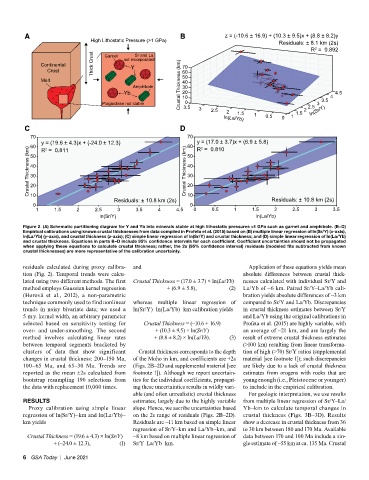
Figure 2. (A) Schematic partitioning diagram for Y and Yb into minerals stable at high lithostatic pressures >1 GPa such as garnet and amphibole. (B–D)
Empirical calibrations using known crustal thicknesses from data compiled in Profeta et al. (2015) based on (B) multiple linear regression of ln(Sr/Y) (x-axis),
ln(La/Yb) (y-axis), and crustal thickness (z-axis); (C) simple linear regression of ln(Sr/Y) and crustal thickness; and (D) simple linear regression of ln(La/Yb)
and crustal thickness. Equations in parts B–D include 95% confidence intervals for each coefficient. Coefficient uncertainties should not be propagated
when applying these equations to calculate crustal thickness; rather, the 2s (95% confidence interval) residuals (modeled fits subtracted from known
crustal thicknesses) are more representative of the calibration uncertainty.

residuals calculated during proxy calibra- and Application of these equations yields mean
tion (Fig. 2). Temporal trends were calcu- absolute differences between crustal thick-
lated using two different methods. The first Crustal Thickness = (17.0 ± 3.7) × ln(La/Yb) nesses calculated with individual Sr/Y and
method employs Gaussian kernel regression + (6.9 ± 5.8), (2) La/Yb of ~6 km. Paired Sr/Y–La/Yb cali-
(Horová et al., 2012), a non-parametric bration yields absolute differences of ~3 km
technique commonly used to find nonlinear whereas multiple linear regression of compared to Sr/Y and La/Yb. Discrepancies
trends in noisy bivariate data; we used a ln(Sr/Y)–ln(La/Yb)–km calibration yields in crustal thickness estimates between Sr/Y
5 m.y. kernel width, an arbitrary parameter and La/Yb using the original calibrations in
selected based on sensitivity testing for Crustal Thickness = (−10.6 ± 16.9) Profeta et al. (2015) are highly variable, with
over- and under-smoothing. The second + (10.3 ± 9.5) × ln(Sr/Y) an average of ~21 km, and are largely the
method involves calculating linear rates + (8.8 ± 8.2) × ln(La/Yb). (3) result of extreme crustal thickness estimates
between temporal segments bracketed by (>100 km) resulting from linear transforma-
clusters of data that show significant Crustal thickness corresponds to the depth tion of high (>70) Sr/Y ratios (supplemental
changes in crustal thickness: 200–150 Ma, of the Moho in km, and coefficients are ±2s material [see footnote 1]); such discrepancies
100–65 Ma, and 65–30 Ma. Trends are (Figs. 2B–2D and supplemental material [see are likely due to a lack of crustal thickness
reported as the mean ±2s calculated from footnote 1]). Although we report uncertain- estimates from orogens with rocks that are
bootstrap resampling 190 selections from ties for the individual coefficients, propagat- young enough (i.e., Pleistocene or younger)
the data with replacement 10,000 times. ing these uncertainties results in wildly vari- to include in the empirical calibration.
able (and often unrealistic) crustal thickness For geologic interpretation, we use results
RESULTS estimates, largely due to the highly variable from multiple linear regression of Sr/Y–La/
Proxy calibration using simple linear slope. Hence, we ascribe uncertainties based Yb–km to calculate temporal changes in
regression of ln(Sr/Y)–km and ln(La/Yb)– on the 2s range of residuals (Figs. 2B–2D). crustal thickness (Figs. 3B–3D). Results
km yields Residuals are ~11 km based on simple linear show a decrease in crustal thickness from 36
regression of Sr/Y–km and La/Yb–km, and to 30 km between 180 and 170 Ma. Available
Crustal Thickness = (19.6 ± 4.3) × ln(Sr/Y) ~8 km based on multiple linear regression of data between 170 and 100 Ma include a sin-
+ (−24.0 ± 12.3), (1) Sr/Y–La/Yb–km. gle estimate of ~55 km at ca. 135 Ma. Crustal

6 GSA Today | June 2021