Introduction
Since William Smith’s iconic geological map of England and Wales in 1815 (Sharpe, 2015), stratigraphic
correlation has become the integral method to decipher and contextualize Earth’s history. Stratigraphic
correlation is now facilitated by sophisticated ancillary measurements of sedimentary rocks, including stable
isotope composition (e.g., McKinney et al., 1950; Knoll et al., 1986), trace element concentration (e.g., Veizer
and Compston, 1974; Elderfield, 1986), and properties such as gamma-ray spectrometry (e.g., Chamberlain, 1984;
Cowan and Myers, 1988) and magnetostratigraphy (e.g., Opdyke, 1972; Løvlie, 1989). Computational advances have
led to quantitative tools for time-series analysis of these ancillary measurements (e.g., Agterberg and
Gradstein, 1988; Tipper, 1988), including software for the correlation of biostratigraphic (e.g., Kemple et al.,
1995; Sadler, 2004; Sadler et al., 2009), paleomagnetic (e.g., Clark, 1985; Hagen et al., 2020),
lithostratigraphic (e.g., Lewis et al., 2011), cyclostratigraphic (e.g., Meyers, 2014; Li et al., 2019), ice
core (e.g., Bay et al., 2010; Hagen and Harper, 2023), and chemostratigraphic data (e.g., Lisiecki and Lisiecki,
2002; Hay et al., 2019). Many of these correlation tools utilize dynamic time warping (DTW), an objective, time
normalization algorithm that achieves least-squares alignments between two time-series. These alignments are
subject to penalties on the insertion of hiatuses that stretch and squeeze the stratigraphic height/time axis
(hence the colloquial term “dynamic time warping”; Sakoe and Chiba, 1978). For two geoscience examples, Lisiecki
and Raymo (2005) adopted the Match algorithm of Lisiecki and Lisiecki (2002) to generate the canonical “LR04”
stack of 57 Pliocene–Pleistocene benthic oxygen isotope records (although, in this case, manual adjustments were
made after applying the algorithm), and the well-resolved Ordovician and Silurian time scales arose from dynamic
programming-based constrained optimization (CONOP) for the temporal sequencing (or “slotting”) of graptolite
first/last appearance datums (Sadler, 2004; Sadler and Cooper, 2008).
Despite the ubiquitous application of chemostratigraphy for stratigraphic correlation across the geological
time scale, and this rich archive of algorithms, the stratigraphy community lacks an open-source code for a free
programming environment to facilitate quantitative chemostratigraphic alignment that is operable by users
without prior coding experience. Here we present Align (Fig. 1), a new free and open-source computer
app that utilizes the DTW algorithm of Hay et al. (2019). Align is available to download from the
GitHub data repository1 and was written in R v.4.2.2 (R Core Team, 2022) using the Shiny
open-source package (Chang et al., 2017). Align utilizes the Hay et al. (2019) DTW algorithm
(originally written in MATLAB), rewritten in R to run seamlessly with the app (Hagen, 2023). We chose to make
the DTW algorithm of Hay et al. (2019) accessible for three reasons. First, this routine efficiently aligns
every individual data point, rather than blocks of data (as the Match algorithm does). Second, the code
generates a library of optimal alignments (in a least-squares sense) between two univariate stratigraphic
time-series data sets. These alignments are subject to systematic assumptions about the total temporal overlap
between the two time-series and the extent to which they can be stretched or squeezed (“time-warped”) to align
with one another (see mathematical description below). This type of analysis is impossible to achieve with the
human eye. Third, the code can be applied to any numerical (though not categorical) stratigraphic time-series
data set (see GitHub repository for a description of how to upload and review data with Align). The
Align interface utilizes intuitive design features such as drop-down menus, slider control elements,
and toggle buttons for the execution of the underlying DTW code without any coding. Here we present a guide for
applying the Align app to time-uncertain chemostratigraphic correlation by demonstrating the alignment
of stable carbon isotope data from carbonate rocks (δ13Ccarb). We provide a description of
the underlying mathematics of DTW.
Uploading, Viewing, Storing, and Culling the Library of Stratigraphic Alignments
The Align interface allows a user to upload spreadsheets of up to three univariate candidate
time-series data sets and a single univariate target time-series data set against which to align the
candidate(s) (formatting details are in the Align documentation on GitHub). Figure 1 illustrates how
the algorithm aligns a synthetic δ13Ccarb data set with a –5‰ excursion followed by a –1‰
excursion, both from a background value of 0‰ (Fig. 1A, target; from Trampush and Hajek [2017]), and a synthetic
δ13Ccarb data set made by randomly subsampling the target (at 20% completeness) and adding
noise (Fig. 1A, candidate) to represent a realistic record that a stratigrapher might correlate. A button
generates a plot of the uploaded δ13Ccarb time-series records to verify accurate data
upload and to cache necessary files for the DTW algorithm (Fig. 1A). At this stage, the user slides bars to set
the range of edge and g values (which control the temporal overlap and relative accumulation
rate, respectively, as discussed below) that determine the size of the alignment library (# of alignments = # of
edge values × # of g values). After plotting verification, the user clicks the “Run DTW
algorithm” button to command the underlying R code to generate the alignment library.
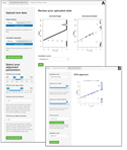 Figure
1
Figure
1
The
Align app for stratigraphic time-series alignment. (A) A screenshot of the
Align graphical
user interface (tab 1) where menus (on left) prompt the user to upload, plot, and align a target and a candidate
time-series data set using the underlying dynamic time-warping (DTW) algorithm. The example target data set
“Synthetic TH17” (adopted from Trampush and Hajek, 2017) and candidate data set “Noisy subsample” (see GitHub
repository [text footnote 1]) are plotted with a click button (on right) to visually confirm accurate data
upload. (B) A screenshot of the
Align culling interface (tab 2) where sliding scales (on left) allow a
user to narrow the resulting alignment libraries by the Pearson correlation coefficient (“xc cutoff”) and/or
overlap percent cutoffs. The example criteria (xc cutoff = 0.9; overlap cutoff = 90%) narrow the full library of
60 alignments down to nine alignments. The user can use a drop-down menu to plot one of these alignments at a
time (on right).
The Align app allows the user to vary the g and edge parameter in any continuous
range between 0.95 and 1.05 and 0.01 and 0.25, respectively, with any increment; following Hay et al. (2019),
the default g value range is set to 0.98–1.01 and the default edge value range is set to
0.01–0.15, both in increments of 0.01. As the underlying code runs through the default parameter space, it
generates 60 alignments (60 g-edge pairings for each candidate-target time-series correlation), which
are visually presented as x-y scatterplots of δ13Ccarb-stratigraphic height (Fig. 1B) and
corresponding spreadsheets containing the meterage that every candidate time-series
δ13Ccarb value was aligned to on the target time-series (i.e., the y-axis values for the
aligned candidate). A different parameter range and increment will change the number of alignments in the
alignment library, and the associated output images/files (see GitHub repository for additional discussion about
g and edge values, as well as hiatal surfaces and data types). Output files are saved to the
user’s computer in a folder named Output with sub-directories named for the candidate-target alignment pair.
Each alignment can be viewed in the underlying Output_Images folder (or plotted in an external application using
the .csv files in the underlying Output_Data folder). A subset of output alignments can be viewed in the
separate alignment library viewer tab (Fig. 1B).
When a stratigrapher wants to focus on a subset of alignments that adhere to a shared criterion, a separate tab
in the Align app gives the user the option to manually sort (and narrow) the alignment library
according to thresholds for the Pearson’s correlation coefficient and the overlap between the aligned
time-series (Fig. 1B). Figure 1B shows the Align interface for culling an alignment library, here
displayed to cull the alignment library to show only those alignments with a Pearson correlation coefficient
≥0.9 (“xc cutoff”) and an overlap of the candidate to the target of ≥90% “overlap cutoff”. When the user clicks
the “Narrow Alignment Library” button (Fig. 1B), Align saves those alignments that adhere to the cutoff
criteria (a “culled library”) in a new folder named for the user’s inputted name for these culling criteria
(e.g., 0.9,90%). For this scenario, the culled alignment library includes nine of the original 60 alignments
(the culled alignments can be viewed independently by selecting their name in the drop-down menu; Fig. 1B).
Relative temporal constraints on stratigraphic sections (e.g., biostratigraphy, litho-stratigraphic markers,
etc.) can be used in conjunction with the time-series data to evaluate an alignment library. For one, the user
can restrict the target/candidate time-series to a certain biozone or lithostratigraphic unit (effectively
aligning δ13Ccarb data presumed to be temporally equivalent). Alternatively, these
constraints can be used to evaluate the alignment libraries post analysis.
How Dynamic Time Warping Produces a Library of Stratigraphic Alignments
Figure 2 illustrates a simple stratigraphic correlation using DTW with two short, synthetic carbon isotope
(δ13Ccarb) time-series: a seven-sample target sequence composed of a 3.5‰
δ13Ccarb excursion over 6 m of stratigraphy (Fig. 2H) and a four-sample candidate sequence
with a 4.5‰ excursion over 3 m (Fig. 2H). First, target (Figs. 1A and 2A) and candidate (Figs. 1A and 2B)
matrices are constructed whose number of rows (n = 7) and columns (m = 4) equal the length of
the target and candidate δ13Ccarb sequences, respectively. The seven
δ13Ccarb values from the target section fill target matrix column 1 (Fig. 2A, red column)
and are replicated m-1 times to fill all remaining columns. The four δ13Ccarb
values from the candidate section are transposed to fill candidate matrix row 1 and replicated n-1
times to fill the remaining rows (Fig. 2B). The next step is to construct an n-by-m matrix of
all of the possible δ13Ccarb pairings from the target and candidate sequences. Each matrix
element is computed as the difference between an index in the target (tn) and the candidate
(cm) sequences: C(n,m) = (tn – cm; Fig. 2C) and squared to give a
squared-difference matrix (Fig. 2D; Sakoe and Chiba, 1978). Comparison of the 3‰ excursion peak in the target
(Fig. 2A, row 4) and candidate sequences (Fig. 2B, column 2) gives a strong constraint because it alone gives a
squared difference of 0 (Fig. 2D, cell (4,2)).
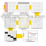 Figure 2
Illustration of the dynamic time warping technique for aligning simple, synthetic δ
13C
carb
sequences. (A–G) Step-by-step matrix operations to align the two synthetic δ
13C
carb
sequences (target, original candidate) shown in frame (H). The target and original candidate
δ
13C
carb sequences populate the columns and rows of the target (A) and candidate (B)
matrices, respectively; subtracting the candidate matrix from the target matrix yields the difference matrix
(C). Squaring the values in the difference matrix generates the squared-difference matrix (D), a measure of the
similarity of all pairs of δ
13C
carb from the target and candidate sections. Multiplying
the edges of the squared-difference matrix by the adopted value of the edge parameter yields the
edge-modified matrix (E). The cumulative difference matrix (F) incorporates the accumulation of cost
arising from the adopted value of the
g parameter. The alignment path, which reveals the temporally
equivalent target and candidate strata/δ
13C
carb values, begins in the lower right corner
of the cumulative difference matrix and proceeds to the lowest cost cell looking two steps ahead (G). For these
synthetic data, the alignment path shifts the aligned candidate section stratigraphically higher on the target
sequence relative to the original candidate meterage (H). Abbreviations: Difference = the difference matrix; Sq.
Diff. = the squared-difference matrix; min(aug. 8 preceding) = the minimum value of the eight preceding
cumulative difference matrix cells;
Edge = the
edge-modified matrix.
An alignment takes the form of a “warping path” that assigns each candidate index m to an index
n of the target sequence by minimizing the sum of the squared differences (“cost”) across all
m (Sakoe and Chiba, 1978). This path is achieved through successive diagonal, horizontal, and vertical
steps across the squared-difference matrix, each of which implies a bed-to-bed alignment (Hay et al., 2019). A
warping path that begins in the lower-right corner of the squared-difference matrix (Fig. 2D, cell (7,4))
implies that the stratigraphically highest δ13Ccarb value from both the target and
candidate sections are time equivalent. A warping path that exits the upper-left corner of the
squared-difference matrix (Fig. 2D, cell (1,1)) aligns the lowermost values of the two sequences, implying that
accumulation began concurrently at both sections. Thus, a warping path that enters and exits both corners of the
squared-difference matrix indicates that sediment accumulation at the two sections spans the same interval of
geological time. In contrast, when a warping path meets an edge of the squared-difference matrix, this implies
that the two sections do not span the same total temporal duration.
Once the warping path enters the matrix, the DTW algorithm objectively finds an optimal pathway in terms of a
sequence of diagonal, vertical, and horizontal steps that minimize the associated sum of squared residuals. A
diagonal step implies an equivalent rate of relative sediment accumulation between the candidate and
target time-series. A vertical or horizontal step instead inserts a hiatus in deposition at the candidate or
target sections, respectively.
When aligning δ13Ccarb sequences, stratigraphers have little or no a priori
information about the total temporal overlap with the target section, nor the relative rates of sediment
accumulation between target and candidate sections. To address these uncertainties, the algorithm explores
various optimal warping paths across the squared-difference matrix (e.g., Fig. 2G) conditional on the systematic
application of the edge and g penalty functions (see below) that alter the values of the
squared-difference matrix (Fig. 2D) and thereby favor specific stratal pairings.
The edge penalty function explores whether the two sequences span the same total interval of time and is so
named because the right and bottom squared-difference matrix edges align the stratigraphically highest
(youngest) target and candidate δ13Ccarb values whereas the left and top edges align the
lowest (oldest) δ13Ccarb values. The edge value is a coefficient that modifies
all squared-difference matrix edge cells in clockwise fashion, beginning with the first row and ending with the
first column (Fig. 2E; yellow ellipsoids). Edge values >1 increase the value of the squared
difference for a specific stratal pairing, discouraging their alignment, whereas when 0 < edge <
1,
stratal pairings are encouraged. For example, an (arbitrarily adopted) edge value of 0.1 modifies
squared-difference matrix element (3,4) = 9 (Fig. 2D) to the lower value of 0.9 (Fig. 2E, cell (3,4)). In this
formulation, matrix corners are modified twice (once per edge; see Fig. 2E, cell (1,1)). While Figure 2
illustrates the adoption of a single (arbitrary) edge value (edge = 0.1; Fig. 2E), in
practice the DTW algorithm systematically varies edge values across a user-identified range to discover
alternative start/end cells for warping pathways, generating multiple δ13Ccarb alignments.
The g penalty function is useful for enforcing various levels of similarity of sediment accumulation
rate(s) at the two stratigraphic sections throughout their shared deposition history using a range of g
values. Values of g > 1 penalize stretching or squeezing by increasing the augmented cost of all
off-diagonal matrix cells, and the opposite is true for g < 1; a g-value equal to 1 does
not augment the cost matrix. For this illustration, we adopt g = 1. First, edge-modified
matrix cell (1,1; Fig. 2E) is replicated to fill the corresponding cell of the cumulative difference matrix
(CDM; Fig. 2F). Next, moving right across CDM row 1, every cell value is computed as the sum of values of the
corresponding edge-modified matrix cell plus all preceding edge-modified matrix cells in the
row (Fig. 2F; horizontal black arrow). For example, CDM (1,4; Fig. 2F) is calculated as the sum of
edge-modified matrix (1,4), (1,3), (1,2), and (1,1), equal to 0.01, 0, 1.225, and 0.0025, respectively,
or 1.2375 (Fig. 2F). This process is repeated vertically for CDM column 1, summing down the column (Fig. 2F;
vertical black arrow).
Next, the algorithm calculates the accumulation of cost in each unfilled cell of row 2 and in each unfilled
cell of column 2 (Fig. 2F; yellow arrows). These values are computed as the sum of the value in the
corresponding edge-modified matrix cell (Fig. 2E) and the minimum value of the three preceding
g-modified cells of the CDM computed as: g*(n, m-1), (n-1, m-1),
and g*(n-1, m) (Fig. 2F; note that three preceding cells are considered only for cell
calculations in row 2 and column 2, whereas cell calculations in all subsequent rows and columns consider eight
preceding cells). For example, the algorithm computes CDM cell (7,2) as the sum of edge-modified matrix
(7,2) = 1.6 (Fig. 2E) and the minimum of the three preceding CDM cells, in this case element (6,1) = 3.1275,
yielding 4.7275 (Fig. 2F). Figure 2 adopts g = 1 for mathematical ease; had we adopted any g ≠
1, this selection would have modified cell (7,1)—calculated as g*(n, m-1)—to be a
value less than cell (6,1)—unmodified by g based on its diagonal position—and thereby changed the final
value for CDM cell (7,2). Like the edge parameter, the DTW algorithm systematically varies g
values
across a user-defined range to discover alternative warping paths between given start/end cells.
To complete the CDM, the algorithm fills the remaining empty cells in rows 3–7 and columns 3–4 (Fig. 2F; gray
arrows). These calculations proceed by summing the corresponding edge-modified matrix value and the
minimum value of the eight preceding CDM cells (looking two steps forward is preferred, considering the
eight preceding cells, but this is not possible in row 2 and column 2 due to the dimensions of the matrix and
there being no 0th row or column, hence the consideration of only three preceding cells representing one step
forward in row 2 and column 2). The CDM cells are modified by g as follows: (n-1, m) and
(n, m-1) are multiplied by g; (n-1, m-2) and (n-2, m-1)
are multiplied by 1.05*g; (n-2, m) and (n, m-2) are multiplied by
1.1*g (Fig. 2F). Diagonal preceding cells (n-1, m-1) and (n-2, m-2)
are not modified by g. For example, CDM cell (3,4) is computed as edge-modified matrix (3,4) = 0.9
(Fig. 2E) plus CDM (1,2) = 1.2275 (because this cell has the minimum value of the eight preceding cells in the
CDM: (3,2), (3,3), (2,2), (2,3), (2,4), (1,2), (1,3), and (1,4)), summing to 2.1275 (Fig. 2F).
Every possible pairing of g and edge values from the input ranges produces a CDM, and the
warping path across the CDM begins at the lower-right corner and progressively steps horizontally, diagonally,
or vertically (see the illustrative alignment in Fig. 2) to the minimum value of the eight adjacent cells,
always looking two steps ahead (Fig. 2G, black cells, with values replicated from Fig. 2F). For each CDM, the
corresponding δ13Ccarb alignment begins with the stratigraphically lowest cell of the
starting edge (the right column or bottom row)—here cell (6,4; Fig. 2G)—and terminates upon meeting an end edge
(the left column/top row), here cell (2,1). Note when the algorithm encounters equivalent values, such as cells
(6,1) and (7,1), the diagonal is adopted to maximize temporal correspondence by minimizing the insertion of
hiatuses. For the adopted edge and g parameter values, the warping path specifies the globally
optimal alignment of each δ13Ccarb value of the candidate sequence with the target
sequence (black cells), with empty rows representing target δ13Ccarb values with no
time-equivalent at the candidate section (an imposed hiatus). Figure 2H visualizes the target-candidate
δ13Ccarb alignment arising from the alignment path in Figure 2G (i.e., for edge
and g values of 0.1 and 1, respectively). By repeating this process for a range of edge and
g values, the algorithm systematically generates alignments that encapsulate a spectrum of assumptions
about the shared temporal history (via edge) and relative rates of sediment accumulation (via
g) at the target
and candidate stratigraphic sections (see Hay et al., 2019). A different pairing of edge and g
values can produce a visually distinct alignment from that shown in Figure 2H (e.g., choosing a g value
greater than 1, which encourages dissimilar relative sedimentation rates, could increase the overlap of the
shoulders of the synthetic excursion). Together, we present the objective alignments arising from all
edge and g pairings as a correlation library for further parsing by statistical analyses and
geological insight (see GitHub repository for a brief discussion of computation time and dynamic programming).
Summary
The user-friendly Align app makes freely available the proven DTW algorithm for objective,
reproducible, and optimal stratigraphic time-series correlation (Hay et al., 2019) to anyone conducting
stratigraphic research by eliminating the need for command-line coding. The Align app efficiently (~1
minute run time) and systematically generates a library of stratigraphic alignments for the stratigrapher to
evaluate, a task otherwise impossible with the human eye. Align allows the user to cull an alignment
library and saves all outputs in common file formats easily read into figure-design software, making
Align a powerful new stratigraphy research tool. We welcome collaborations to incorporate additional
features into Align to grow the capacity of this community tool.
Acknowledgments
We thank the DTW algorithm creators (C. Hay and E. Haam), app beta-testers (S. Herz, M. Schwarz, A. Martin, and
R. Jones), and P. Reynolds and K. Jay for feedback. Financial support from the NSF GRFP, ARCS Foundation,
Agouron Institute Geobiology Fellowship, and NSF EAR-2025735 made this work possible. We thank James Schmitt for
editorial handling, as well as Benjamin Gill and an anonymous reviewer whose constructive feedback greatly
improved this manuscript.
References Cited
- Agterberg, F.P., and Gradstein, F.M., 1988, Recent developments in quantitative stratigraphy: Earth-Science
Reviews, v. 25, p. 1–73, https://doi.org/10.1016/0012-8252(88)90099-2.
- Bay, R.C., Rohde, R.A., Price, P.B., and Bramall, N.E., 2010, South Pole paleowind from automated synthesis
of ice core records: Journal of Geophysical Research: Atmospheres, v. 115,
https://doi.org/10.1029/2009JD013741.
- Chamberlain, A.K., 1984, Surface gamma-ray logs: A correlation tool for frontier areas: AAPG Bulletin, v.
68, p. 1040–1043, https://doi.org/10.1306/AD4616C4-16F7-11D7-8645000102C1865D.
- Chang, W., Cheng, J., Allaire, J., Xie, Y., and McPherson, J., 2017, Shiny: Web application
framework for R: R package version, v. 1, https://CRAN.R-project.org/package=shiny.
- Clark, R.M., 1985, A FORTRAN program for constrained sequence-slotting based on minimum combined path
length: Computers & Geosciences, v. 11, p. 605–617, https://doi.org/10.1016/0098-3004(85)90089-5.
- Cowan, D.R., and Myers, K.J., 1988, Surface gamma-ray logs: A correlation tool for frontier areas:
Discussion: AAPG Bulletin, v. 72, p. 634–636.
- Elderfield, H., 1986, Strontium isotope stratigraphy: Palaeogeography, Palaeoclimatology, Palaeoecology, v.
57, p. 71–90, https://doi.org/10.1016/0031-0182(86)90007-6.
- Hagen, C.J., 2023, Align: A Modified DTW Algorithm for Stratigraphic Time-Series Alignment:
https://cran.r-project.org/package=align (accessed 30 June 2023).
- Hagen, C.J., and Harper, J.T., 2023, Dynamic time warping to quantify age distortion in firn cores impacted
by melt processes: Annals of Glaciology, https://doi.org/10.1017/aog.2023.52.
- Hagen, C.J., Reilly, B.T., Stoner, J.S., and Creveling, J.R., 2020, Dynamic time warping of palaeomagnetic
secular variation data: Geophysical Journal International, v. 221, p. 706–721,
https://doi.org/10.1093/gji/ggaa004.
- Hay, C.C., Creveling, J.R., Hagen, C.J., Maloof, A.C., and Huybers, P., 2019, A library of early Cambrian
chemostratigraphic correlations from a reproducible algorithm: Geology, v. 47, p. 457–460,
https://doi.org/10.1130/G46019.1.
- Kemple, W.G., Sadler, P.M., and Strauss, D.J., 1995, Extending Graphic Correlation to Many Dimensions:
Stratigraphic Correlation as Constrained Optimization:
https://archives.datapages.com/data/sepm_sp/SP53/Extending_Graphic_Correlation_to_Many_Dimensions.htm
(accessed February 2023).
- Knoll, A.H., Hayes, J.M., Kaufman, A.J., Swett, K., and Lambert, I.B., 1986, Secular variation in carbon
isotope ratios from Upper Proterozoic successions of Svalbard and East Greenland: Nature, v. 321, p. 832–838,
https://doi.org/10.1038/321832a0.
- Lewis, K.W., Keeler, T.L., and Maloof, A.C., 2011, New software for plotting and analyzing stratigraphic
data: Eos, v. 92, p. 37–38, https://doi.org/10.1029/2011EO050002.
- Li, M., Hinnov, L., and Kump, L., 2019, Acycle: Time-series analysis software for paleoclimate
research and education: Computers & Geosciences, v. 127, p. 12–22,
https://doi.org/10.1016/j.cageo.2019.02.011.
- Lisiecki, L.E., and Lisiecki, P.A., 2002, Application of dynamic programming to the correlation of
paleoclimate records: Paleoceanography, v. 17, p. 1-1–1-12,https://doi.org/10.1029/2001PA000733.
- Lisiecki, L.E., and Raymo, M.E., 2005, A Pliocene-Pleistocene stack of 57 globally distributed benthic
δ18O
records: Paleoceanography, v. 20, https://doi.org/10.1029/2004PA001071.
- Løvlie, R., 1989, Paleomagnetic stratigraphy: A correlation method: Quaternary International, v. 1, p.
129–149, https://doi.org/10.1016/1040-6182(89)90012-8.
- McKinney, C.R., McCrea, J.M., Epstein, S., Allen, H.A., and Urey, H.C., 1950, Improvements in mass
spectrometers for the measurement of small differences in isotope abundance ratios: The Review of Scientific
Instruments, v. 21, p. 724–730, https://doi.org/10.1063/1.1745698.
- Meyers, S.R., 2014, Astrochron: An R package for astrochronology:
https://cran.r-project.org/package=astrochron.
- Opdyke, N.D., 1972, Paleomagnetism of deep-sea cores: Reviews of Geophysics, v. 10, p. 213–249,
https://doi.org/10.1029/RG010i001p00213.
- Sadler, P.M., 2004, Quantitative biostratigraphy: Achieving finer resolution in global correlation: Annual
Review of Earth and Planetary Sciences, v. 32, p. 187–213,
https://doi.org/10.1146/annurev.earth.32.101802.120428.
- Sadler, P.M., and Cooper, R.A., 2008, Best-fit intervals and consensus sequences, in Harries, P.J.,
ed., High-Resolution Approaches in Stratigraphic Paleontology: Dordrecht, Netherlands, Springer, p. 49–94,
https://doi.org/10.1007/978-1-4020-9053-0_2.
- Sadler, P.M., Cooper, R.A., and Melchin, M., 2009, High-resolution, early Paleozoic (Ordovician-Silurian)
time scales: Geological Society of America Bulletin, v. 121, p. 887–906, https://doi.org/10.1130/B26357.1.
- Sakoe, H., and Chiba, S., 1978, Dynamic programming algorithm optimization for spoken word recognition: IEEE
Transactions on Acoustics, Speech, and Signal Processing, v. 26, p. 43–49,
https://doi.org/10.1109/TASSP.1978.1163055.
- Sharpe, T., 2015, The birth of the geological map: Science, v. 347, p. 230–232,
https://doi.org/10.1126/science.aaa2330.
- Team, R.C., 2022, R: A language and environment for statistical computing: R Foundation for Statistical
Computing, https://www.R-project.org/.
- Tipper, J.C., 1988, Techniques for quantitative stratigraphic correlation: A review and annotated
bibliography: Geological Magazine, v. 125, p. 475–494, https://doi.org/10.1017/S0016756800013224.
- Trampush, S.M., and Hajek, E.A., 2017, Preserving proxy records in dynamic landscapes: Modeling and examples
from the Paleocene-Eocene Thermal Maximum: Geology, v. 45, p. 967–970, https://doi.org/10.1130/G39367.1.
- Veizer, J., and Compston, W., 1974, 87Sr/86Sr composition of seawater during the
Phanerozoic: Geochimica et
Cosmochimica Acta, v. 38, p. 1461–1484, https://doi.org/10.1016/0016-7037(74)90099-4.