Introduction
The study of Earth’s past relies on a record that is spatially and temporally variable and, by some
metrics, woefully undersampled. Through every geochemical analysis, fossil identification, and measured
stratigraphic section, Earth scientists continuously add to this historical record. Compilations of such
observations can illuminate global trends through time, providing researchers with crucial insights into
our planet’s geological and biological evolution. These compilations can vary in size and scope, from
hundreds of manually curated entries in a spreadsheet to millions of records stored in software
databases. The latter form is exemplified by databases such as The Paleobiology Database (PBDB; Peters
and McClennen, 2016), Macrostrat (Peters et al., 2018), EarthChem (Walker et al., 2005), Georoc (Sarbas,
2008), and the Sedimentary Geochemistry and Paleoenvironments Project (SGP, this study).
Of course, large amounts of data are not new to the Earth sciences, and, with respect to volume, many
Earth history and geochemistry compilations are small in comparison to the datasets used in other
subdisciplines, including seismology (e.g., Nolet, 2012), climate science (e.g., Faghmous and Kumar,
2014), and hydrology (e.g., Chen and Wang, 2018). As a result, many Earth history compilations likely do
not meet the criteria to be called “big data,” which is a term that describes very large amounts of
information that accumulate rapidly and which are heterogeneous and unstructured in form (Gandomi and
Haider, 2015; or “if it fits in memory, it is small data”). That said, the tens of thousands to millions
of entries present in such datasets do represent a new frontier for those interested in our planet’s
past. For many Earth historians, however, and especially for geochemists (where most of the field’s
efforts traditionally have focused on analytical measurements rather than data analysis; see Sperling et
al., 2019), this frontier requires new outlooks and toolkits.
When using compilations to extract global trends through time, it is important to recognize that large
datasets can have several inherent issues. Observations may be unevenly distributed temporally and/or
spatially, with large stretches of time (e.g., parts of the Archean Eon) or space (e.g., much of Africa;
Fig. S11) lacking data. There may also be errors with entries—mislabeled values,
transposition issues, and missing metadata can occur in even the most carefully curated compilations.
Even if data are pristine, they may span decades of acquisition with evolving techniques, such that both
analytical precision and measurement uncertainty are non-uniform across the dataset (Fig. S2 [see
footnote 1]). Careful examination may demonstrate that contemporaneous and co-located observations do
not agree. Additionally, data often are not targeted, such that not every entry may be necessary for (or
even useful to) answering a particular question.
Luckily, these (and other) issues can be addressed through careful processing and analysis, using
well-established statistical and computational techniques. Although such techniques have complications
of their own (e.g., a high degree of comfort with programming often is required to run code
efficiently), they do provide a way to extract meaningful trends from large datasets. No one lab can
generate enough data to cover Earth’s history densely enough (i.e., in time and space), but by
leveraging compilations of accumulated knowledge, and using a well-developed computational pipeline,
researchers can begin to ascertain a clearer picture of Earth’s past.
A Proposed Workflow
The process of transforming entries in a dataset into meaningful trends requires a series of steps, many
with some degree of user decision making. Our proposed workflow is designed with the express intent of
removing unfit data while appropriately propagating uncertainties. First, a compiled dataset is made or
sourced (Fig. S3, i. [see footnote 1]). Next, a researcher chooses between in-database analysis and
extracting data into another format, such as a text file (Fig. S3, ii.). This choice does nothing to the
underlying data—its sole function is to recast information into a digital format that the researcher is
most comfortable with. Then, a decision must be made about whether to remove entries that are not
pertinent to the question at hand (Fig. S3, iii.). Using one or more metadata parameters (e.g., in the
case of rocks, lithological descriptions), researchers can turn large compilations into targeted
datasets, which then can be used to answer specific questions without the influence of irrelevant data.
Following this gross filtering, researchers must decide between removing outliers or keeping them in the
dataset (Fig. S3, iv.). Outliers have the potential to drastically skew results in misleading ways.
Ascertaining which values are outliers is a non-trivial task, and all choices about outlier exclusion
must be clearly described when presenting results. Finally, samples are drawn from the filtered dataset
(i.e., “resampling”) using a weighting scheme that seeks to address the spatial and temporal
heterogeneities—as well as analytical uncertainties—of the data (Fig. S3, vi.). To calculate statistics
from the data, multiple iterations of resampling are required.
Case Study: The Sedimentary Geochemistry and Paleoenvironments Project
The SGP project seeks to compile sedimentary geochemical data, made up of various analytes (i.e.,
components that have been analyzed), from throughout geologic time. We applied our workflow to the SGP
database2 to extract coherent temporal trends in Al2O3 and U from
siliciclastic mudstones. Al2O3 is relatively immobile and thus useful for
constraining both the provenance and chemical weathering history of ancient sedimentary deposits (Young
and Nesbitt, 1998). Conversely, U is highly sensitive to redox processes. In marine mudstones, U serves
as both a local proxy for reducing conditions in the overlying water column (i.e., authigenic U
enrichments only occur under low-oxygen or anoxic conditions and/or very low sedimentation rates; see
Algeo and Li, 2020) and a global proxy for the areal extent of reducing conditions (i.e., the magnitude
of authigenic enrichments scales in part with the global redox landscape; see Partin et al., 2013).
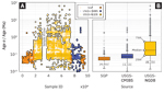
SGP data are stored in a PostgreSQL relational database that currently comprises a total of 82,579
samples (Fig. 1). The SGP database was created by merging sample data and geological context information
from three separate sources, each with different foci and methods for obtaining the “best guess” age of
a sample (i.e., the interpreted age as well as potential maximum and minimum ages). The first source is
direct entry by SGP team members, which focuses primarily on Neoproterozoic–Paleozoic shale samples and
has global coverage. Due to the direct involvement of researchers intimately familiar with their sample
sets, these data have the most precise (Fig. 1A)—and likely also most accurate—age constraints. Second,
the SGP database has incorporated sedimentary geochemical data from the United States Geological Survey
(USGS) National Geo-chemical Database (NGDB), comprising samples from projects completed between the
1960s and 1990s. These samples, which cover all lithologies and are almost entirely from Phanerozoic
sedimentary deposits of the United States, are associated with the continuous-time age model from
Macrostrat (Peters et al., 2018). Finally, the SGP database includes data from the USGS Global
Geochemical Database for Critical Metals in Black Shales project (CMIBS; Granitto et al., 2017), culled
to remove ore-deposit related samples. The CMIBS samples predominantly are shales, have global coverage,
and span the entirety of Earth’s sedimentary record. When possible, the CMIBS data are associated with
Macrostrat continuous-time age models; otherwise, the data are assigned age information by SGP team
members (albeit without detailed knowledge of regional geology or geologic units).
 Figure
1
Figure
1
Visualizations of data in the Sedimentary Geochemistry and Paleoenvironments Project (SGP) database. (A)
Relative age uncertainty (i.e., the reported age σ divided by the reported interpreted age) versus
Sample ID. The large gap in Sample ID values resulted from the deletion of entries during the initial
database compilation and has no impact on analyses. (B) Box plot showing the distributions of relative
ages with respect to the sources of data. CMIBS—Critical Metals in Black Shales; NGDB—National
Geochemical Database.
Cleaning and Filtering
We exported SGP data into a comma-separated values (.csv) text file, using a custom structured query
language (SQL) query. In the case of geochemical analytes, this query included unit conversions from
both weight percent (wt%) and parts per billion (ppb) to parts per million (ppm). After export, we
parsed the .csv file and screened the data through a series of steps. First, if multiple values were
reported for an analyte in a sample, we calculated and stored the mean (or weighted mean, if there were
enough values) and standard deviation of the analyte. Then, we redefined empty values—which are the
result of abundance being above or below detection—as “not a number” (NaN, a special value defined by
Institute of Electrical and Electronics Engineers [IEEE] floating-point number standard that always
returns false on comparison; see IEEE, 2019). Next, we converted major elements (e.g., those that
together comprise >95% of Earth’s crust or individually >1 wt% of a sample) into their
corresponding oxides; if an oxide field did not already exist, or if there was no measurement for a
given oxide, the converted value was inserted into the data structure. Then, we assigned both age and
measurement uncertainties to the parsed data. In the case of the parsed SGP data, 5,935 samples (i.e.,
7.1% of the original dataset) lacked an interpreted age and so no uncertainty could be assigned. For the
remainder, we calculated an initial absolute age uncertainty by either using the reported maximum and
minimum ages:
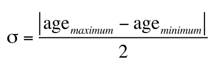
,
or, if there were no maximum and minimum age values available, by defaulting to a two-sigma value of 6%
of the interpreted age:
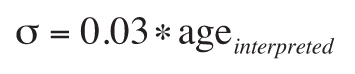
.
The choice of a 6% default value was based on a conservative estimate of the precision of common in situ
dating techniques (see, for example, Schoene, 2014). Additionally, we enforced a minimum σ of 25 million
years:
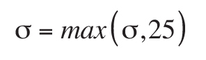
.
Effectively, each datum can be thought of as a Gaussian distribution along the time axis with a σ of at
least 25 million years (the minimum value of which may be thought of as a kernel bandwidth, rather than
an analytical uncertainty). The selection of this σ value should correspond to an estimate of the
processes that are being investigated (e.g., tectonic changes in provenance). We did not impose a
minimum relative age uncertainty.
With respect to measurement uncertainties, we assigned an absolute uncertainty to every analyte that
lacked one by multiplying the reported analyte value by a relative error. In future database projects,
there is considerable scope to go beyond this coarse uncertainty quantification strategy. For example,
given the detailed metadata associated with each sample in the SGP database, it would be straightforward
to develop correction factors or uncertainty estimates for different geochemical methodologies (e.g.,
inductively coupled plasma–mass spectrometry [ICP-MS] versus inductively coupled plasma–optical emission
spectrometry [ICP-OES], benchtop versus handheld X-ray fluorescence spectrometry [XRF], etc.).
Correcting data for biases introduced during measurement is common in large Earth science datasets (Chan
et al., 2019). However, such corrections previously have not been attempted in sedimentary geochemistry
datasets.
Next, we processed the data through a simple lithology filter because, in the general case of rock-based
datasets, only lithologies relevant to the question(s) at hand provide meaningful information. The
choice of valid lithologies (or, for that matter, any other filterable metadata) are dependent on the
researchers’ question(s). As highlighted in the Discussion section, lithology filtering has significant
implications for redox-sensitive and/or mobile/immobile elements. In this case study, our aim was to
only sample data generated from siliciclastic mudstones. To decide which values to screen by, we
manually examined a list made up of all unique lithologies in the dataset. We excluded samples that did
not match our list of chosen lithologies (removing ~63.5% of the data; Table S1; Fig. S4 [see footnote
1]). Our strategy ensured that we only included mudstones sensu lato (see Potter et al., 2005, for a
general description) where the lithology was coded. Alternative methods—such as choosing samples based
on an Al cutoff value (e.g., Reinhard et al., 2017)—likely would result in a set comprising both
mudstone and non-mudstone coded lithologies. In the future, improved machine learning algorithms,
designed to classify unknown samples based on their elemental composition, may provide a more
sophisticated means by which to generate the largest possible dataset of lithology-appropriate samples.
We then completed a preliminary screening of the lithology filtered samples by checking if extant analyte
values were outside of physically possible bounds (e.g., individual oxides with wt% less than 0 or
greater than 100), and, if so, setting them to NaN. Next, to reduce the number of mudstone samples with
detrital or authigenic carbonate and phosphatic mineral phases, we excluded samples with greater than 10
wt% Ca and/or more than 1 wt% P2O5 (removing ~66.9% of the remaining data; Fig. S4
[see footnote 1]). Additionally, in order to ensure that our mudstone samples were not subject to
secondary enrichment processes, such as ore mineralization, we queried the USGS NGDB to extract the
recorded characteristics of every sample with an associated USGS NGDB identifier. We examined these
characteristics for the presence of selected strings (i.e., “mineralized,” “mineralization present,”
“unknown mineralization,” and “radioactive”) and excluded any sample exhibiting one or more strings.
Finally, as there were still several apparent outliers in the dataset, we manually examined the log
histograms of each element and oxide of interest. On each histogram, we demarcated the 0.5th and 99.5th
percentile bounds of the data, then visually studied those histograms to exclude “outlier populations,”
or samples located both well outside those percentile bounds and not part of a continuum of values
(removing ~5.7% of the remaining data; Fig. S4). Following these filtering steps, we saved the data in a
.csv text file.
Data Resampling
We implemented resampling based on inverse distance weighting (after Keller and Schoene, 2012), in which
samples closer together—that is, with respect to a metric such as age or spatial distance—are considered
to be more alike than samples that are further apart. The inverse weighting of an individual point, x,
is based on the basic form:
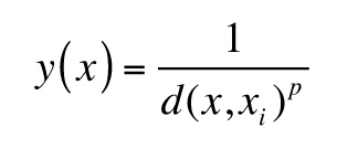
,
where d is a distance function, xi is a second sample, and p, which
is greater than 0, is a power parameter. In the case of the SGP data, we used two distance functions,
spatial (s) and temporal (t):
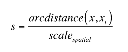
,
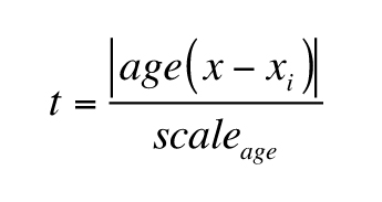
,
where arcdistance refers to the distance between two points on a sphere,
scalespatial refers to a preselected arc distance value (in degrees; Fig. S5, inset
[see footnote 1]), and scaleage is a preselected age value (in million years, Ma).
In this case study, we chose a scalespatial of 0.5 degrees and a
scaleage of 10 Ma (see below for a discussion about parameter values).
For n samples, the proximity value w assigned to each sample x is:
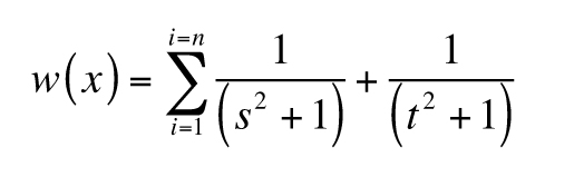
.
Essentially, the proximity value is a summation of the reciprocals of the distance measures made for each
pair of the sample and a single other datum from the dataset. Accordingly, samples that are closer to
other data in both time and space will have larger w values than those that are farther away.
Note that the additive term of 1 in the denominator establishes a maximum value of 1 for each reciprocal
distance measure.
We normalized the generated proximity values (Fig. S6 [see footnote 1]) to produce a probability value
P. This normalization was done such that the median proximity value corresponded to a
P of ~0.20 (i.e., a 1 in 5 chance of being chosen):
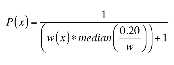
.
This normalization results in an “inverse proximity weighting,” such that samples that are closer to
other data (which have large w values) end up with a smaller P value than those that
are far away from other samples. Next, we assigned both analytical and temporal uncertainties to each
analyte to be resampled. Then, we culled the dataset into an m by n matrix, where each
row corresponded to a sample and each column to an analyte. We resampled this culled dataset 10,000
times using a three-step process: (1) we drew samples, using calculated P values, with
replacement (i.e., each draw considered all available samples, regardless of whether a sample had
already been drawn); (2) we multiplied the assigned uncertainties discussed above by a random draw from
a normal distribution (µ = 0; σ = 1) to produce an error value; and (3) we added these newly calculated
errors to the drawn temporal and analytical values. Finally, we binned and plotted the resampled data.
Naturally, the reader may ask how we chose the values for scaleage and
scaletemporal and what, if any, impact those choices had on the final results?
Nominally, the values of scaleage and scaletemporal are
controlled by the size and age, respectively, of the features that are being sampled. So, in the case of
sedimentary rocks, those values should reflect the length scale and duration of a typical sedimentary
basin, such that many samples from the same “spatiotemporal” basin have lower P values than few
samples from distinct basins. Of course, it is debatable what “typical” means in the context of
sedimentary basins, as both size and age can vary over orders of magnitude (Woodcock, 2004). Given this
uncertainty, we subjected the SGP data to a series of sensitivity tests, where we varied both
scaleage and scaletemporal, using logarithmically spaced values
of each (Fig. S5 [see footnote 1]). While the uncertainty associated with results varied based on the
choice of the two parameters, the overall mean values were not appreciably different (Fig. S7 [see
footnote 1]).
Results
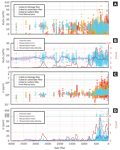
To study the impact of our methodology, we present results for two geochemical components, U and
Al2O3 (Fig. 2). Contents-wise, the U and Al2O3 data in the
SGP database contain extreme outliers. Many of these outliers were removed using the lithology and Ca or
P2O5 screening (Figs. 2A and 2C); the final outlier filtering strategy discussed
above handled any remaining values of concern. In the case of U, our multi-step filtering reduced the
range of concentrations by three orders of magnitude, from 0–500,000 ppm to 0–500 ppm.
 Figure
2
Figure
2
Filtering and resampling of Al
2O
3 and U. (A) and (C). Al
2O
3
and U data through time, respectively. Each datum is color coded by the filtering step at which it was
separated from the dataset. In blue is the final filtered data, which was used to generate the resampled
trends in (B) and (D). (B) and (D). Plots depicting Al
2O
3 and U filtered data,
along with a histogram of resampled data density and the resulting resampled mean and 2σ error. Note
the log-scale y axis in (C).
Discussion
The illustrative examples we have presented have implications for understanding Earth’s history.
Al2O3 contents of ancient mudstones appear relatively stable over the past ca.
1500 Ma (the time interval for which appreciable data exist in our dataset), suggesting little
first-order change in Al2O3 delivery to sedimentary basins over time. The U
contents of mudstones shows a substantial increase between the Proterozoic and Phanerozoic. Although we
have not accounted for the redox state of the overlying water column, these results broadly recapitulate
the trends seen in a previous much smaller (and non-weighted) dataset (Partin et al., 2013) and
generally may indicate oxygenation of the oceans within the Phanerozoic.
Moving forward, there is no reason to believe that the compilation and collection of published data,
whether in a semi-automated (e.g., SGP) or automated (e.g., GeoDeepDive; Peters et al., 2014) manner,
will slow and/or stop (Bai et al., 2017). Those interested in Earth’s history—as collected in large
compilations—should understand how to extract meaningful trends from these ever-evolving datasets. By
presenting a workflow that is purposefully general and must be adapted before use, we hope to elucidate
the various aspects that must be considered when processing large volumes of data.
Foremost to any interpretation of a quantitative dataset is an assessment of uncertainty. In truth, a
datum representing a physical quantity is not a single scalar point, but rather, an entire distribution.
In many cases, such as in our workflow, this distribution is implicitly assumed to be Gaussian, an
assumption that may or may not be accurate (Rock et al., 1987)—although a simplified distribution
certainly is better than none. The quantification of uncertainty in Earth sciences especially is
critical when averaging and binning by a selected independent variable, since neglecting the uncertainty
of the independent variable will lead to interpretational failures that may not be mitigated by adding
more data. As time perhaps is the most common independent variable (and one with a unique relationship
to the assessment of causality), incorporating its uncertainty especially is critical for the purposes
of Earth history studies (Ogg et al., 2016). An age without an uncertainty is not a meaningful datum.
Indeed, such a value is even worse than an absence of data, for it is actively misleading. Consequently,
assessment of age uncertainty is one of the most important, yet underappreciated, components of building
accurate temporal trends from large datasets.
Of course, age is not the only uncertain aspect of samples in compiled datasets, and researchers should
seek to account for as many inherent uncertainties as possible. Here, we propagate uncertainty by using
a resampling methodology that incorporates information about space, time, and measurement error. Our
chosen methodology—which is by no means the only option available to researchers studying large
datasets—has the benefit of preventing one location or time range from dominating the resulting trend.
For example, although the Archean records of Al2O3 and U especially are sparse
(Fig. 2), resampling prevents the appearance of artificial “steps” when transitioning from times with
little data to instances of (relatively) robust sampling (e.g., see the resampled record of
Al2O3 between 4000 and 3000 Ma). Therefore, researchers should examine their
selected methodologies to ensure that: (1) uncertainties are accounted for, and (2) that spatiotemporal
heterogeneities are addressed appropriately.
Even with careful uncertainty propagation, datasets must also be filtered to keep outliers from affecting
the results. It is important to note that the act of filtering does not mean that the filtered data are
necessarily “bad,” just that they do not meaningfully contribute to the question at hand. For example,
while our lithology and outlier filtering methods removed most U data because they were inappropriate
for reconstructing trends in mudstone geochemistry through time, that same data would be especially
useful for other questions, such as determining the variability of heat production within shales. This
sort of filtering is a fixture of scientific research—e.g., geochemists will consider whether samples
are diagenetically altered when measuring them for isotopic data—and, likewise, should be viewed as a
necessary step in the analysis of large datasets.
As our workflow demonstrates, filtering often requires multiple steps, some automatic (e.g., cutoffs that
exclude vast amounts of data in one fell swoop or algorithms to determine the “outlierness” of data; see
Ptáček et al., 2020) and others manual (e.g., examining source literature to determine whether an
anomalous value is, in fact, meaningful). Each procedure, along with any assumptions and/or
justifications, must be documented clearly (and code included and/or stored in a publicly accessible
repository) by researchers so that others may reproduce their results and/or build upon their
conclusions with increasingly larger datasets.
Along with documentation of data processing, filtering, and sampling, it is important for researchers
also to leverage sensitivity analyses to understand how parameter choices may impact resulting trends.
Here, through the analysis of various spatial and temporal parameter values, we demonstrate that, while
the spread of data varies based on the prescribed values of scalespatial and
scaletemporal, the averaged resampled trend does not (Fig. S7 [see footnote 1]). At
the same time, we see that trends are directly influenced by the use (or lack thereof) of Ca and
P2O5 and outlier filtering. For example, the record of U in mudstones becomes
overprinted by anomalously large values when carbonate samples are not excluded (Fig. S7B).
Conclusions
Large datasets can provide increasingly valuable insights into the ancient Earth system. However, to
extract meaningful trends, these datasets must be cultivated, curated, and processed with an emphasis on
data quality, uncertainty propagation, and transparency. Charles Darwin once noted that the “natural
geological record [is] a history of the world imperfectly kept” (Darwin, 1859, p. 310), a reality that
is the result of both geological and sociological causes. But while the data are biased, they also are
tractable. As we have demonstrated here, the challenges of dealing with this imperfect record—and, by
extension, the large datasets that document it—certainly are surmountable.
Acknowledgments
We thank everyone who contributed to the SGP database, including T. Frasier (YGS). BGS authors (JE, PW)
publish with permission of the Executive Director of the British Geological Survey, UKRI. We would like
to thank the editor and one anonymous reviewer for their helpful feedback.
References Cited
- Algeo, T.J., and Li, C., 2020, Redox classification and calibration of redox thresholds in
sedimentary systems: Geochimica et Cosmochimica Acta, v. 287, p. 8–26,
https://doi.org/10.1016/j.gca.2020.01.055.
- Bai, Y., Jacobs, C.A., Kwan, M., and Waldmann, C., 2017, Geoscience and the technological revolution
[perspectives]: IEEE Geoscience and Re-mote Sensing Magazine, v. 5, no. 3, p. 72–75,
https://doi.org/10.1109/MGRS.2016.2635018.
- Chan, D., Kent, E.C., Berry, D.I., and Huybers, P., 2019, Correcting datasets leads to more
homogeneous early-twentieth-century sea surface warming: Nature, v. 571, no. 7765, p. 393–397,
https://doi.org/10.1038/s41586-019-1349-2.
- Chen, L., and Wang, L., 2018, Recent advances in Earth observation big data for hydrology: Big Earth
Data, v. 2, no. 1, p. 86–107, https://doi.org/10.1080/20964471.2018.1435072.
- Darwin, C., 1859, On the Origin of Species by Means of Natural Selection, or Preservation of
Favoured Races in the Struggle for Life: London, John Murray, 490 p.
- Faghmous, J.H., and Kumar, V., 2014, A big data guide to understanding climate change: The case for
theory-guided data science: Big Data, v. 2, no. 3, p. 155–163,
https://doi.org/10.1089/big.2014.0026.
- Gandomi, A., and Haider, M., 2015, Beyond the hype: Big data concepts, methods, and analytics:
International Journal of Information Manage-ment, v. 35, no. 2, p. 137–144,
https://doi.org/10.1016/j.ijinfomgt.2014.10.007.
- Granitto, M., Giles, S.A., and Kelley, K.D., 2017, Global Geochemical Database for Critical Metals
in Black Shales: U.S. Geological Survey Data Release, https://doi.org/10.5066/F71G0K7X.
- IEEE, 2019, IEEE Standard for Floating-Point Arithmetic: IEEE Std 754-2019 (Revision of IEEE
754-2008), p. 1–84, https://doi.org/10.1109/IEEESTD.2008.4610935.
- Keller, C.B., and Schoene, B., 2012, Statistical geochemistry reveals disruption in secular
lithospheric evolution about 2.5 gyr ago: Nature, v. 485, no. 7399, p. 490–493,
https://doi.org/10.1038/nature11024.
- Nolet, G., 2012, Seismic tomography: With applications in global seismology and exploration
geophysics: Berlin, Springer, v. 5, 386 p., https://doi.org/10.1007/978-94-009-3899-1.
- Ogg, J.G., Ogg, G.M., and Gradstein, F.M., 2016, A concise geologic time scale 2016: Amsterdam,
Elsevier, 240 p.
- Partin, C.A., Bekker, A., Planavsky, N.J., Scott, C.T., Gill, B.C., Li, C., Podkovyrov, V., Maslov,
A., Konhauser, K.O., Lalonde, S.V., Love, G.D., Poulton, S.W., and Lyons, T.W., 2013, Large-scale
fluctuations in Precambrian atmospheric and oceanic oxygen levels from the record of U in shales:
Earth and Planetary Science Letters, v. 369, p. 284–293, https://doi.org/10.1016/j.epsl.2013.03.031.
- Peters, S.E., and McClennen, M., 2016, The paleobiology database application programming interface:
Paleobiology, v. 42, no. 1, p. 1–7, https://doi.org/10.1017/pab.2015.39.
- Peters, S.E., Zhang, C., Livny, M., and Re, C., 2014, A machine reading system for assembling
synthetic paleontological databases: PLOS One, v. 9, no. 12, e113523,
https://doi.org/10.1371/journal.pone.0113523.
- Peters, S.E., Husson, J.M., and Czaplewski, J., 2018, Macrostrat: A platform for geological data
integration and deep-time Earth crust research: Geochemistry Geophysics Geosystems, v. 19, no. 4, p.
1393–1409, https://doi.org/10.1029/2018GC007467.
- Potter, P.E., Maynard, J.B., and Depetris, P.J., 2005, Mud and Mudstones: Introduction and Overview:
Berlin, Springer, 297 p.
- Ptáček, M.P., Dauphas, N., and Greber, N.D., 2020, Chemical evolution of the continental crust from
a data-driven inversion of terrigenous sedi-ment compositions: Earth and Planetary Science Letters,
v. 539, p. 116090.
- Reinhard, C.T., Planavsky, N.J., Gill, B.C., Ozaki, K., Robbins, L.J., Lyons, T.W., Fischer, W.W.,
Wang, C., Cole, D.B., and Konhauser, K.O., 2017, Evolution of the global phosphorus cycle: Nature,
v. 541, no. 7637, p. 386–389, https://doi.org/10.1038/nature20772.
- Rock, N.M.S., Webb, J.A., McNaughton, N.J., and Bell, G.D., 1987, Nonparametric estimation of
averages and errors for small data-sets in isotope geoscience: A proposal: Chemical Geology, Isotope
Geoscience Section, v. 66, no. 1–2, p. 163–177.
- Sarbas, B., 2008, The Georoc database as part of a growing geoinformatics network, in
Geoinformatics 2008—Data to Knowledge: U.S. Geological Survey, p. 42–43.
- Schoene, B., 2014, U-Th-Pb geochronology, in Holland, H.D., and Turekian, K.K., eds.,
Treatise on Geochemistry (Second Edition): Oxford, UK, Elsevier, p. 341–378.
- Sperling, E.A., Tecklenburg, S., and Duncan, L.E., 2019, Statistical inference and reproducibility
in geobiology: Geobiology, v. 17, no. 3, p. 261–271, https://doi.org/10.1111/gbi.12333.
- Walker, J.D., Lehnert, K.A., Hofmann, A.W., Sarbas, B., and Carlson, R.W., 2005, EarthChem:
International collaboration for solid Earth geo-chemistry in geoinformatics: AGUFM, v. 2005,
IN44A-03.
- Woodcock, N.H., 2004, Life span and fate of basins: Geology, v. 32, no. 8, p. 685–688,
https://doi.org/10.1130/G20598.1.
- Young, G.M., and Nesbitt, H.W., 1998, Processes controlling the distribution of Ti and Al in
weathering profiles, siliciclastic sediments and sedi-mentary rocks: Journal of Sedimentary
Research, v. 68, no. 3, p. 448–455.