
Full Text View
Volume 25 Issue 8 (August 2015)
GSA Today
![]()
Article, pp. 4-10 | Abstract | PDF (5.9MB)
Pleistocene relative sea levels in the Chesapeake Bay region and their implications for the next century
| Table of Contents |
|---|
|
Search GoogleScholar for
Search GSA Today |
ABSTRACT
Today, relative sea-level rise (3.4 mm/yr) is faster in the Chesapeake Bay region than any other location on the Atlantic coast of North America, and twice the global average eustatic rate (1.7 mm/yr). Dated interglacial deposits suggest that relative sea levels in the Chesapeake Bay region deviate from global trends over a range of timescales. Glacio-isostatic adjustment of the land surface from loading and unloading of continental ice is likely responsible for these deviations, but our understanding of the scale and timeframe over which isostatic response operates in this region remains incomplete because dated sea-level proxies are mostly limited to the Holocene and to deposits 80 ka or older.
To better understand glacio-isostatic control over past and present relative sea level, we applied a suite of dating methods to the stratigraphy of the Blackwater National Wildlife Refuge, one of the most rapidly subsiding and lowest-elevation surfaces bordering Chesapeake Bay. Data indicate that the region was submerged at least for portions of marine isotope stage (MIS) 3 (ca. 60–30 ka), although multiple proxies suggest that global sea level was 40–80 m lower than present. Today MIS 3 deposits are above sea level because they were raised by the Last Glacial Maximum forebulge, but decay of that same forebulge is causing ongoing subsidence. These results suggest that glacio-isostasy controlled relative sea level in the mid-Atlantic region for tens of thousands of years following retreat of the Laurentide Ice Sheet and continues to influence relative sea level in the region. Thus, isostatically driven subsidence of the Chesapeake Bay region will continue for millennia, exacerbating the effects of global sea-level rise and impacting the region’s large population centers and valuable coastal natural resources.
*Emails: DeJong: ; Bierman: ; Newell: ; Rittenour: ; Mahan: ; Balco: ; Rood:
DOI: 10.1130/GSATG223A.1
Manuscript received 1 July 2014; accepted 12 Jan. 2015.
Introduction
The sea level for any location at a given point in time represents a sum of factors, including the volume of ocean water, steric (thermal) effects, tectonic activity, and crustal deformation in response to glacio-hydro-isostatic adjustment (GIA) from loading and unloading of continental ice and water masses (Church et al., 2010). GIA can be a dominant driver of relative sea level (RSL) near ice margins, where the weight of ice displaces the mantle beneath glaciated regions, uplifting a “forebulge” in the peripheral, non-glaciated region (Peltier, 1986). With ice retreat, the forebulge progressively subsides at rates dependent on mantle rheology and lithosphere thickness (Peltier, 1996).
GIA played a role in RSL near the Chesapeake Bay region of the United States (Fig. 1) for many millennia after the ice melted away (Peltier, 2009). GIA effects were first recognized in the region when shoreline deposits ~3–5 m above present sea level, long assumed to be ca. 125 ka (marine isotope stage [MIS] 5e; MIS designations from Lisiecki and Raymo, 2005), were found to have ca. 80 ka ages (MIS 5a; Cronin, 1981). During this time, global average sea level was as much as 20 m below its present level (Fig. 2). While flexural isostatic uplift and subsidence have been documented in the Chesapeake Bay region (i.e., Pazzaglia and Gardner, 1993), the rates (~0.006 mm/yr) associated with these processes are insufficient to account for the age-elevation relationships of MIS 5a shorelines.
|
Map showing Atlantic coast of the United States with population density by county (U.S. Census Bureau, 2010) placed alongside Late Holocene and twentieth-century relative sea-level rise (RSL) rise curves (2 errors; Engelhart et al., 2009). RSL rise predicted from glacio-hydro-isostatic adjustment (GIA) modeling is from the M2 viscosity model (Peltier, 1996). Yellow shaded region brackets area of highest RSL rise on the Atlantic coast; dotted white line indicates maximum extent of the Laurentide ice sheet (LIS) (Dyke et al., 2002); magenta lines indicate tracks of major recent storms. PL, S, MP—Locations of coastal deposits dating to MIS 3 near central Chesapeake Bay (67–37 ka, n = 8; Pavich et al., 2006; Litwin et al., 2013), in southern Virginia (50–33 ka, n = 2; Scott et al., 2010), and North Carolina (59–28 ka, n = 15; Mallinson et al., 2008, Parham et al., 2013), respectively. A–A´ shows location of Figure 2A. |
 Figure 1
|
(A) Schematic cross section showing relationship of land surface to relative sea level at specific times in glacial cycles as a function of distance from the Laurentide ice sheet (LIS). Adapted by permission from D. Krantz and C. Hobbs (2014, pers. comm.). Location of A–A´ cross section is indicated in Figure 1. (B) Oxygen isotope and sea-level curves for the past 150 k.y. from Lisiecki and Raymo (2005) and Thompson and Goldstein (2006), respectively. The glacioisostatic (land surface) curve (after Scott et al., 2010) is based on ages produced for shoreline deposits in the mid-Atlantic region and illustrates how land-surface elevation change induced by glacio-hydro-isostatic adjustment can account for submergence of the Chesapeake Bay region when eustatic sea level was much lower than present. VPDB—Vienna Pee Dee Belemnite. |
 Figure 2
The presence of MIS 5a shorelines 3–5 m above present sea level indicates that the land surface within the Chesapeake Bay region was significantly lower during the formation of these shorelines due to regional land subsidence from the collapse of the MIS 6 forebulge, and that the Chesapeake Bay region experienced renewed forebulge uplift during the MIS 2 to raise these shorelines above present sea level (Potter and Lambeck, 2003; Wehmiller et al., 2004). The Holocene stratigraphic record in the Chesapeake Bay region helps illuminate forebulge dynamics; differential subsidence from the collapse of the MIS 2 forebulge caused variable timing and rates of inundation along the eastern seaboard during the Holocene transgression (Peltier, 1996). These differential rates have been exploited to reconstruct the form of the fore-bulge (Engelhart et al., 2009) and to constrain GIA models (Fig. 1) (Davis and Mitrovica, 1996; Peltier, 1996).
Recent studies employing optically stimulated luminescence (OSL) dating suggest that the lowest-elevation, emerged estuarine deposits within the mid-Atlantic were deposited during MIS 3, significantly extending the inferred duration and magnitude of land subsidence due to collapse of the MIS 6 forebulge. Shoreline landforms above sea level (<8 m above mean sea level [asl]) near central Chesapeake Bay (PL, Fig. 1), at the mouth of Chesapeake Bay (S, Fig. 1), and on the North Carolina coast (MP, Fig. 1) indicate estuarine deposition throughout MIS 3 (67–32 ka). Eustatic sea level during this time was highly variable but always ~40–80 m lower than present (Fig. 2) (Siddall et al., 2008). These new data challenge the long-held implication that locations within the Chesapeake Bay region, and specifically the Delmarva Peninsula, did not experience high-stand deposition after MIS 5 (e.g., Ramsey, 2010). The presence of near-shore MIS 3 deposits near present sea level suggests an alternative sea-level history for the region, one that implies forebulge uplift of at least 40 m since the time of deposition. This uplift has been attributed to growth of the last glacial maximum (LGM; MIS 2) forebulge (Pavich et al., 2006; Mallinson et al., 2008; Scott et al., 2010; Parham et al., 2013) that remains uplifted out of isostatic equilibrium (Potter and Lambeck, 2003).
This paper uses multiple methods to date deposits within the zone of greatest subsidence in the Chesapeake Bay region (Fig. 1) and place today’s rapid relative sea-level rise into the context of a several-million-year geologic framework. We used a light detection and ranging (LiDAR) digital elevation model (DEM) to analyze low-relief landforms and conducted extensive drilling to constrain the Pleistocene stratigraphic framework. Our data show that regional subsidence related to collapse of the MIS 6 glacio-isostatic forebulge impacted the mid-Atlantic region well into MIS 3, tens of thousands of years after MIS 5 deglaciation. Long-lasting subsidence associated with collapse of the MIS 6 forebulge suggests that present-day subsidence related to the collapse of the MIS 2 forebulge will continue for the foreseeable future. We conclude that ongoing subsidence adds to the impacts of sea-level rise driven by warming climate and melting ice sheets and should be considered in coastal sea-level risk assessments.
Study Site and Methods
To reconstruct the sea-level history in Chesapeake Bay, we focused on the Blackwater National Wildlife Refuge (~110 km2; red-bordered rectangle on Fig. 1), which experienced major inundation and transformation of wetlands to open water in the twentieth century (Fig. 3). Sediment from 70 boreholes was described, analyzed, and sampled. The DEM (Fig. 4) was used to characterize the geomorphology. We constrained the oldest erosional event preserved directly above the underlying Miocene strata using cosmogenic nuclide isochron burial dating (Balco and Rovey, 2008). We dated 28 samples using optically stimulated luminescence (OSL) dating. The OSL ages allow us to develop a geochronological framework for the Blackwater National Wildlife Refuge landforms and estuarine sediments to a depth of ~9 m (Fig. 5). Eight radiocarbon dates constrain the timing of Holocene inundation and the beginning of marsh accretion. Detailed methods are provided in the online GSA Supplemental Data Repository 1 .
|
Time series of the Blackwater River valley. Top: Intact marsh surveyed from AD 1902 to AD 1904 and presented in a 7.5˝ USGS topographic map from AD 1905 (USGS, 1905); dark blue hatching around the Blackwater valley is tidal marsh; light blue pattern is freshwater swamp. Middle: Initiation of major ponding seen in an aerial photograph from 1938 (http://www.esrgc.org/). Bottom: Coalesced ponds forming the informal “Lake Blackwater” in satellite imagery from AD 2007 (http://www.bing.com/maps/). Wetlands are converting to open water at a rate of 50–150 ha/yr in the field area (Cahoon et al., 2010). Image locations are identified in Figure 4B. Red outline shows location of unnamed island for reference. |
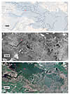 Figure 3
|
(A) LiDAR-derived digital elevation model (DEM) of the Blackwater National Wildlife Refuge projected with the NAD83 datum; produced by H. Pierce (2012, pers. comm.); m ASL—meters above sea level. Cell size is 2.5 m by 2.5 m; graduated elevation scale indicated to the left of the image exaggerates subtle features in the lowest elevation ranges. White outline indicates boundary of the Blackwater National Wildlife Refuge. (B) Same LiDAR DEM as (A) in gray-scale with geomorphic features referenced in the text superimposed. AD 1905 channel margins were digitized from the topographic map in Figure 3A. |
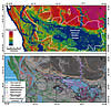 Figure 4
|
(A) Cross section showing the Pleistocene deposits that underlie the Blackwater National Wildlife Refuge. All ages are in thousands of years (ka). Italicized ages are cosmogenic burial isochrons; underlined ages are radiocarbon ages; all others are optically stimulated luminescence ages. Yellow shading represents Holocene deposits; green shading represents MIS 5 and MIS 3 deposits; shades of red, orange, and blue indicate three distinct paleochannel systems, with depths of western channels inferred from boreholes drilled off the line of section; gray substrate is the Miocene Chesapeake Group. Note break in vertical scale. See Fig. 4B for B–B´ line of section. See GSA Supplemental Data Figures S4 and S5 (see footnote 1) for more detail on sedimentology. |
__________
1 GSA supplemental data item 2015211, data tables and methodology, is online. You can also request a copy from GSA Today, P.O. Box 9140, Boulder, CO 80301-9140, USA; .
Results and Interpretations
The Blackwater National Wildlife Refuge is underlain by Pleistocene deposits that vary in thickness from ~3–55 m (Fig. 5). Glacial-interglacial climate fluctuations induced major cycles of localized river incision and aggradation in the Chesapeake Bay region (Colman et al., 1990), and the subsurface Blackwater National Wildlife Refuge stratigraphy includes cut-fill deposits associated with at least three paleochannel systems (Fig. 5). Isochron ages at the base of the Pleistocene section are 1.72 ± 0.08 Ma for a Susquehanna River paleochannel and 2.06 ± 0.14 Ma for a local paleochannel system (2; Fig. 5 and GSA Supplemental Data Table S1 [see footnote 1]). The older age indicates that major cutting and filling commenced in the study area shortly after the onset of major Northern Hemisphere continental glaciation (2.4 Ma; Balco and Rovey, 2010). These ages are significantly older than previous age estimates for paleochannels of the Chesapeake Bay (ca. 18–450 ka; Colman et al., 1990). The complex Pleistocene stratigraphic record and age range of material overlying these dated deposits suggest that fluvio-estuarine processes dominated landscape evolution over glacial-interglacial timescales in the field area (Fig. 5).
LiDAR allows us to identify a variety of landforms on the Blackwater National Wildlife Refuge surface that form a continuum with the shallow stratigraphy (<12 m depth; Figs. 4 and 5). A regressive, wave-cut scarp with multiple bifurcations (beach ridges, Fig. 4B) separates upland areas to the north and east from the lower terrain in the south and west that is occupied by an expansive tidal marsh. These shoreline features consist of an ~3 m fining upward sequence of burrowed, silty fine sand to massive, medium sand (GSA Supplemental Data Fig. S5 [see footnote 1]) with an age range of 53–40 ka (n = 6; see Fig. 5 and GSA Supplemental Data Table S2). Below the scarp, large subaqueous bars (Fig. 4B) that roughly parallel the paleo-shoreline dominate the geomorphology. The bars consist of facies ranging from horizontally bedded, alternating sand and silt to moderately sorted, fine-to-medium sand interpreted as wave-sorted tidal channel deposits and wave-built bars within tidal tributaries or bays. OSL ages for surficial landforms below the scarp range from 69 to 35 ka (n = 15). The morphology, lithology, and ages of these features indicate that estuarine conditions prevailed, at least intermittently, during most of MIS 3, with active bar migration continuing during regression. Locally, unconformities separate multiple, stacked MIS 3 deposits, and in some locations MIS 3 deposits cut older estuarine units that were dated to both MIS 5a and MIS 5e (Fig. 5; GSA Supplemental Data Figs. S4 and S5 [see footnote 1]).
The MIS 3 estuarine surface is truncated by a north-south–trending, meandering channel with scroll bars as well as elliptical depressions interpreted as ephemeral basins (Fig. 4B). The rims of basins are composed of laminated, silty, fine-to-medium sand with ages 30–26 ka (n = 3); the meandering channel must be younger than the ca. 35 ka sand bars it cuts. The basins and channel are likely relict from periglacial processes that dominated this landscape beginning ca. 30 ka and continued through the LGM (Denny et al., 1979; Newell and Clark, 2008; French et al., 2009; Markewich et al., 2009; Newell and DeJong, 2011; Gao, 2014).
Sediments from the Holocene transgression (yellow, Fig. 5) overlap MIS 3 estuarine deposits within incised valleys of the Blackwater River and its tributaries. They consist of a lower silt (~3–4 m) with locally abundant organic material that transitions to an upper, dense, organic peat (~3–4 m). A radiocarbon (14C) age from woody material near the base of the silt (-8.5 m) suggests initial Holocene transgression into the Blackwater River valley by 5310–5570 cal yr B.P. Woody material within the silt, just below the peat boundary, is 690–910 cal yr B.P., setting a maximum age for marsh accretion. Radiocarbon samples collected above this boundary and within the peat have modern ages (GSA Supplemental Data Table S3 [see footnote 1]).
Discussion
Fluctuating sea levels, resulting from changes in eustatic sea level, and crustal deformation (uplift and subsidence) related to GIA, define the Pleistocene history of the Blackwater National Wildlife Refuge and the greater Chesapeake Bay region. The Pleistocene record and cosmogenic ages suggest that the onset of Northern Hemisphere glaciation at the Plio-Pleistocene boundary initiated cycles of incision and deposition. The paleo–Susquehanna River and its tributaries responded to repeated ~50–100-m sea-level fluctuations (Lisiecki and Raymo, 2005) with deep incision of river valleys during glacial lowstands and fluvio-estuarine deposition during transgressions. Estuarine conditions prevailed during portions of MIS 3, when global proxies indicate that eustatic sea level was ~40–80 m below present, suggesting prolonged relaxation of a MIS 6 forebulge during MIS 3.
Temperatures and sea levels plunged prior to ca. 30 ka, from their already low MIS 3 levels (Lambeck et al., 2014) (Fig. 2). As the LIS grew, so did the forebulge that uplifted the Chesapeake Bay region through the LGM, likely contributing to rapid incision documented along the Susquehanna and Potomac Rivers (Reusser et al., 2004) as the Chesapeake Bay region was transformed into a periglacial landscape. During the Holocene, the forebulge progressively subsided, as indicated by differential timing of Holocene inundation and variable rates of sea-level rise along the U.S. Atlantic Coast (Engelhart et al., 2009). The Blackwater River valley was inundated by ca. 5 ka, initiating deposition of bay bottom silt. Widespread marshes were established sometime within the last millennium and accreted, keeping pace with sea-level rise. RSL rise accelerated along the U.S. Atlantic coast during the twentieth century (Engelhart et al., 2009), resulting in inundation, erosion, and ponding in the Blackwater National Wildlife Refuge as sea-level rise outpaced marsh accretionary processes (Fig. 3) (Stevenson et al., 2002).
The presence of MIS 3 estuarine deposits near today’s sea level confirms the effects of GIA over long timescales for the Blackwater National Wildlife Refuge and supports similar interpretations within the greater Chesapeake Bay region. The elevations of MIS 3 estuarine deposits generally decrease from the Central Delmarva Peninsula southward to North Carolina (Scott et al., 2010); dated, emerged MIS 3 estuarine deposits are not found south of North Carolina. While the maximum elevations of MIS 3 deposits vary (GSA Supplemental Data Fig. S8 [see footnote 1]), decreasing elevations to the south are consistent with the shape of the forebulge based on subsidence rates (Engelhart et al., 2009). High-precision GPS data, though limited to a short time series, also indicate the highest rates of subsidence on the Atlantic coast are centered on the Chesapeake Bay region (Sella et al., 2007; Snay et al., 2007).
Our data support the hypothesis that subsidence in the Chesapeake Bay region is caused by the continued collapse of the MIS 2 forebulge (Potter and Lambeck, 2003). While subsidence rates vary within the Chesapeake Bay region (Fig. 1) (Engelhart et al., 2009), potentially due to local groundwater withdrawal for commercial use (Eggleston and Pope, 2013), the central Delmarva Peninsula has the highest rates of subsidence in the mid-Atlantic region (~1.3–1.7 mm/yr; Engelhart et al., 2009). Parsing GIA-driven subsidence from other RSL drivers is uncertain (e.g., Cronin, 2012), but the agreement of twentieth-century subsidence values calculated from tide gauge records where effects of seasonal and decadal variability are removed (~1.6 mm/yr, Boon et al., 2010) and from dated Holocene deposits (~1.3 mm/yr; Engelhart et al., 2009) from the same location near our study area implies consistency of rates over millennial timescales. Subsidence is thus primarily driven by GIA in the Chesapeake Bay region, which makes RSL rise in the Chesapeake Bay–Washington D.C. area twice the twentieth-century global average rate of sea-level rise (1.7 mm/yr; IPCC, 2013). If timescales of MIS 6 forebulge subsi-dence are used for comparison, subsidence from the LGM forebulge collapse will continue for many more millennia.
Ongoing GIA-driven subsidence in the Chesapeake Bay region challenges a region already threatened by sea-level rise. At the Blackwater National Wildlife Refuge, we use rate consistency to predict ~0.16 m of subsidence for the region in the twenty-first century (using twentieth-century values from Boon and others [2010] that presumably include the effects of groundwater withdrawal). The likely range of average global sea-level rise for the twenty-first century is 0.33–0.82 m, based on a non-aggressive climate mitigation policy (IPCC, 2013). Superimposing this sea-level rise estimate over 0.16 m of subsidence yields a total predicted RSL rise of 0.49–0.98 m for the Blackwater National Wildlife Refuge by AD 2100.
These are minimum estimates; several lines of evidence suggest that sea levels will rise more quickly in the Chesapeake Bay region. Recent tide gauge analyses indicate the acceleration of sea-level rise in the North Atlantic in recent decades, possibly due to dynamic ocean circulation processes (Yin et al., 2010; Boon, 2012; Ezer and Corlett, 2012; Sallenger et al., 2012). If this acceleration continues, it could induce an additional rise of 15 cm for the Chesapeake Bay and Washington D.C. areas by AD 2100 (Yin et al., 2010). Recent evidence also confirms the instability of glaciers in West Antarctica, which has the potential to raise global sea levels significantly, particularly beyond AD 2100 (Joughin et al., 2014; Rignot et al., 2014). As global sea levels rise and the Chesapeake Bay region subsides, storm surges are projected to increase both in frequency (IPCC, 2013) and magnitude (Tebaldi et al., 2012). Superimposing Hurricane Isabel water levels on the range of RSLs we predict for the Cheapeake Bay region would cause a storm tide of ~3.8–4.6 m in Washington D.C. and ~2.8–3.5 m for Chesapeake Bay (NOAA, 2003). Given the location of the Chesapeake Bay region along the path of storms tracking up the Atlantic coast (Fig. 1), increasing RSL rise will further exacerbate already high costs of storm damage, such as the US$65 billion price-tag associated with Hurricane Sandy (NOAA, 2013).
Even the most conservative estimate of projected RSL rise poses significant threats to the Chesapeake Bay region. Bridges, military facilities, national monuments, and portions of the rapid transit system would be flooded in Washington D.C., and ~70,000 residents would be impacted by a 0.4 m rise in sea level (Ayyub et al., 2012). Island communities in Chesapeake Bay are particularly vulnerable to RSL rise. The last two inhabited islands in Chesapeake Bay are ~1 m above sea level; they occupy the same geomorphic surface as the western portion of our field area and will experience similar rates of subsidence. In the Blackwater National Wildlife Refuge, a LiDAR-based inundation study using a conservative model for sea-level rise shows that the majority of tidal marsh will be inundated by AD 2050 (Larsen et al., 2004).
The elevated risk of flooding in the Chesapeake Bay region is already triggering a societal response. At the Blackwater National Wildlife Refuge, managers are designing corridors for the landward migration of habitat through easements and land acquisition to ensure the persistence of tidal marsh beyond AD 2100. Similar options are increasingly limited on other coastlines, where continued development and site modification for housing severely limit the potential for inland migration of habitat, and wetland loss significantly reduces natural buffers to storms in these regions (Titus et al., 2009). Island communities have limited options; some Chesapeake Bay islands have been abandoned due to sea-level rise in the past century (e.g., Gibbons and Nicholls, 2006).
For Washington D.C. and other coastal cities, risk assessment and adaptation planning based on the full range of possible RSL rise scenarios is critical. The analysis by Ayyub et al. (2012) indicates significant losses for Washington D.C. with a rise of 0.4 m, well below the minimum predicted rise of sea level for AD 2100 of 0.49–0.98 m. This analysis under-predicts the most likely RSL rise over the next century, in part because it does not explicitly consider that GIA will drive increased RSL independent of climate change. We conclude that risk assessments and adaptation planning for sea-level rise should consider the full range of sea-level estimates (e.g., Miller et al., 2013) and take local subsidence values into consideration, particularly for high-density population centers like Washington D.C.
Acknowledgments
This research is supported by the U.S. Geological Survey. M. Whitbeck (USFWS) granted access to the Blackwater National Wildlife Refuge. USGS drillers E. Cobbs and J. Grey made this work possible. We thank M. Nelson, A. Benthem, I. Clark, H. Pierce, J. McGeehin, D. Powars, S. Zimmerman, J. Smoot, and D. Granger for help with this research. M. Pavich and one anonymous reviewer reviewed this manuscript.
REFERENCES CITED
- Ayyub, B.M., Braileanu, H.G., and Qureshi, N., 2012, Prediction and impact of sea level rise on properties and infrastructure of Washington, D.C.: Risk Analysis, v. 32, no. 11, p. 1901–1918, doi: 10.1111/j.1539-6924.2011.01710.x.
- Balco, G., and Rovey, C.W., 2008, An isochron method for cosmogenic-nuclide dating of buried soils and sediments: American Journal of Science, v. 308, no. 10, p. 1083–1114, doi: 10.2475/10.2008.02.
- Balco, G., and Rovey, C.W., 2010, Absolute chronology for major Pleistocene advances of the Laurentide Ice Sheet: Geology, v. 38, no. 9, p. 795–798, doi: 10.1130/G30946.1.
- Boon, J.D., 2012, Evidence of sea-level acceleration at U.S. and Canadian tide stations, Atlantic coast, North America: Journal of Coastal Research, v. 285, p. 1437–1445, doi: 10.2112/JCOASTRES-D-12-00102.1.
- Boon, J.D., Brubaker, J.M., and Forrest, D.R., 2010, Chesapeake Bay land subsidence and sea-level change: An evaluation of past and present trends and future outlook: A Report to the Army Corps of Engineers: Virginia Institute of Marine Science Special Report No. 425 in Applied Marine Science and Ocean Engineering, 35 p.
- Cahoon, D.R., Guntnerspergen, G., Baird, S., Nagel, J., Hensel, P., Lynch, J., Bishara, D., Brennand, P., Jones, J., and Otto, C., 2010, Do annual prescribed fires enhance or slow the loss of coastal marsh habitat at Blackwater National Wildlife Refuge?: Final Project Report to Joint Fire Science Program, http://www.firescience.gov/projects/06-2-1-35/project/06-2-1-35_blackwater_burn_final_report_mar_31_2010.pdf (last accessed 26 Mar. 2015).
- Church, J.A., Woodworth, P.L., Aarup, T., and Wildon, W.S., 2010, Understanding Sea-Level Rise and Variability: UK, Wiley-Blackwell, 456 p.
- Colman, S.M., Halka, J.P., Hobbs, C.H., III, Mixon, R.B., and Foster, D.S., 1990, Ancient channels of the Susquehanna River beneath Chesapeake Bay and the Delmarva Peninsula: GSA Bulletin, v. 102, p. 1268–1279, doi: 10.1130/0016-7606(1990)102<1268:ACOTSR>2.3.CO;2.
- Cronin, T.M., 1981, Rates and possible causes of neotectonic vertical crustal movements of the emerged southeastern United States Atlantic Coastal Plain: GSA Bulletin, v. 92, no. 11, p. 812–833, doi: 10.1130/0016-7606(1981)92<812:RAPCON>2.0.CO;2.
- Cronin, T.M., 2012, Rapid sea-level rise: Quaternary Science Reviews, v. 56, p. 11–30, doi: 10.1016/j.quascirev.2012.08.021.
- Davis, J.L., and Mitrovica, J.X., 1996, Glacial isostatic adjustment and the anomalous tide gauge record of eastern North America: Nature, v. 379, p. 331–333, doi: 10.1038/379331a0.
- Denny, C.S., Owens, J.P., Sirkin, L.A., and Rubin, M., 1979, The Parsonsburg Sand in the Central Delmarva Peninsula, Maryland and Delaware: USGS Professional Paper 1067-B, p. B1–B16.
- Dyke, A.S., Andrews, J.T., Clark, P.U., England, J.H., Miller, G.H., Shaw, J., and Veillette, J.J., 2002, The Laurentide and Innuitian ice sheets during the Last Glacial Maximum: Quaternary Science Reviews, v. 21, p. 9–31, doi: 10.1016/S0277-3791(01)00095-6.
- Eggleston, J.E., and Pope, J., 2013, Land Subsidence and Relative Sea-Level Rise in the Southern Chesapeake Bay Region: USGS Circular 1392, 30 p.
- Engelhart, S.E., Horton, B.P., Douglas, B.C., Peltier, W.R., and Tornqvist, T.E., 2009, Spatial variability of late Holocene and 20th century sea-level rise along the Atlantic coast of the United States: Geology, v. 37, no. 12, p. 1115–1118, doi: 10.1130/G30360A.1.
- Ezer, T., and Corlett, W.B., 2012, Is sea level rise accelerating in the Chesapeake Bay? A demonstration of a novel new approach for analyzing sea level data: Geophysical Research Letters, v. 39, no. 19, p. 1–6, doi: 10.1029/2012GL053435.
- French, H., Demitroff, M., and Newell, W.L., 2009, Past permafrost on the mid-Atlantic coastal plain, eastern United States: Permafrost and Periglacial Processes, v. 20, p. 285–294, doi: 10.1002/ppp.659.
- Gao, C., 2014, Relict thermal-contraction-crack polygons and past permafrost south of the Late Wisconsinan glacial limit in the mid-Atlantic coastal plain, USA: Permafrost and Periglacial Processes, p. 144–149.
- Gibbons, S.J.A., and Nicholls, R.J., 2006, Island abandonment and sea-level rise: An historical analog from the Chesapeake Bay, USA: Global Environmental Change, v. 16, no. 1, p. 40–47, doi: 10.1016/j.gloenvcha.2005.10.002.
- IPCC, 2013, Climate change 2013: The physical science basis. Contribution of the Working Group 1 to the Fifth Assessment report of the Intergovernmental Panel on Climate Change: Cambridge, UK, Cambridge University Press, 2216 p.
- Joughin, I., Smith, B.E., and Medley, B., 2014, Marine ice sheet collapse potentially under way for the Thwaites Glacier Basin, West Antarctica: Science, v. 344, 6185, p. 735–738, doi: 10.1126/science.1249055.
- Lambeck, K., Rouby, H., Purcell, A., Sun, Y., and Sambridge, M., 2014, Sea level and global ice volumes from the Last Glacial Maximum to the Holocene: PNAS, v. 111, no. 43, p. 15,296–15,303.
- Larsen, C., Clark, I., Guntenspergen, G.R., Cahoon, D.R., Caruso, V., Hupp, C., and Yanosky, T., 2004, The Blackwater NWR Inundation Model: Rising Sea Level on a Low-lying Coast: USGS Open File Report 04-1302, http://pubs.usgs.gov/of/2004/1302/ (last accessed 11 May 2015).
- Lisiecki, L.E., and Raymo, M.E., 2005, A Pliocene-Pleistocene stack of 57 globally distributed benthic 18O records: Paleoceanography, v. 20, no. 1, p. 1–17, doi: 10.1029/2004PA001071.
- Litwin, R.J., Smoot, J.P., Pavich, M.J., Markewich, H.W., Brook, G., and Durika, N.J., 2013, 100,000-year-long terrestrial record of millennial-scale linkage between eastern North American mid-latitude paleovegetation shifts and Greenland ice-core oxygen isotope trends: Quaternary Research, v. 80, no. 2, p. 291–315, doi: 10.1016/j.yqres.2013.05.003,
- Mallinson, D., Burdette, K., Mahan, S., and Brook, G., 2008, Optically stimulated luminescence age controls on late Pleistocene and Holocene coastal lithosomes, North Carolina, USA: Quaternary Research, v. 69, no. 1, p. 97–109, doi: 10.1016/j.yqres.2007.10.002.
- Markewich, H.W., Litwin, R.J., Pavich, M.J., and Brook, G.A., 2009, Late Pleistocene eolian features in southeastern Maryland and Chesapeake Bay region indicate strong WNW-NW winds accompanied growth of the Laurentide Ice Sheet: Quaternary Research, v. 71, no. 3, p. 409–425, doi: 10.1016/j.yqres.2009.02.001.
- Miller, K.G., Kopp, R.E., Horton, B.P., Browning, J.V., and Kemp, A.C., 2013, A geological perspective on sea-level rise and its impacts along the U.S. mid-Atlantic coast: Earth’s Future, v. 1, no. 1, p. 3–18, doi: 10.1002/2013EF000135.
- Newell, W.L., and Clark, I., 2008, Geomorphic map of Worcester County, Maryland, interpreted from a LiDAR-based digital elevation model: USGS Open File Report 2008-1005, 34 p.
- Newell, W.L., and DeJong, B.D., 2011, Cold-climate slope deposits and landscape modifications of the Mid-Atlantic Coastal Plain, Eastern USA: Geological Society of London Special Publication 354, p. 259–276, doi: 10.1144/SP354.17.
- NOAA, 2003, Storm Data and Unusual Weather Phenomena: National Weather Service, Sept. 2003, http://www.weather.gov/media/lwx/stormdata/storm0903.pdf (last accessed 26 Mar. 2015).
- NOAA, 2013, Billion-Dollar Weather and Climate Disasters: Table of Events: National Climatic Data Center: http://www.ncdc.noaa.gov/billions/events (last accessed 26 Mar. 2015).
- Parham, P.R., Riggs, S.R., Culver, S.J., Mallinson, D.J., Jack Rink, W., and Burdette, K., 2013, Quaternary coastal lithofacies, sequence development and stratigraphy in a passive margin setting, North Carolina and Virginia, USA: Sedimentology, v. 60, no. 2, p. 503–547, doi: 10.1111/j.1365-3091.2012.01349.x.
- Pavich, M.J., Markewich, H.W., and Brook, G.A., 2006, Significance of Kent Island Formation to geomorphic history of the Mid-Atlantic region: Geological Society of America Abstracts with Programs, v. 38, no. 7, p. 226.
- Pazzaglia, F.J., and Gardner, A.S., 1993, Fluvial terraces of the lower Susquehanna River: Geomorphology, v. 8, p. 83–113, doi: 10.1016/0169-555X(93)90031-V.
- Peltier, W.R., 1986, Deglaciation induced vertical motion of the North American continent and transient lower mantle rheology: Journal of Geophysical Research, v. 91, B8, p. 9099–9123, doi: 10.1029/JB091iB09p09099.
- Peltier, W.R., 1996, Global sea level rise and glacial isostatic adjustment: An analysis of data from the east coast of North America: Geophysical Research Letters, v. 23, no. 7, p. 717–720, doi: 10.1029/96GL00848.
- Peltier, W.R., 2009, Closure of the budget of global sea level rise over the GRACE era: The importance of magnitudes of the required corrections for global glacial isostatic adjustment: Quaternary Science Reviews, v. 28, p. 1658–1674, doi: 10.1016/j.quascirev.2009.04.004.
- Potter, E.-K., and Lambeck, K., 2003, Reconciliation of sea-level observations in the Western North Atlantic during the last glacial cycle: Earth and Planetary Science Letters, v. 217, no. 1–2, p. 171–181.
- Ramsey, K.W., 2010, Stratigraphy, correlation, and depositional environments of the middle to late Pleistocene interglacial deposits of southern Delaware: Delaware Geologic Survey Report of Investigations 76, 43 p.
- Reusser, L.J., Bierman, P.R., Pavich, M.J., Zen, E.-a., Larsen, J., and Finkel, R.C., 2004, Rapid Late Pleistocene incision of Atlantic passive-margin river gorges: Science, v. 305, p. 499–502, doi: 10.1126/science.1097780.
- Rignot, E., Mouginot, J., Morlighem, M., Seroussi, H., and Scheuchl, B., 2014, Widespread, rapid grounding line retreat of Pine Island, Thwaites, Smith, and Kohler glaciers, West Antarctica, from 1992 to 2011: Geophysical Research Letters, v. 41, no. 10, p. 3502–3509, doi: 10.1002/2014GL060140.
- Sallenger, A.H., Doran, K.S., and Howd, P.A., 2012, Hotspot of accelerated sea-level rise on the Atlantic coast of North America: Nature Climate Change, v. 2, p. 884–888, doi: 10.1038/nclimate1597.
- Scott, T.W., Swift, D.J.P., Whittecar, G.R., and Brook, G.A., 2010, Glacioisostatic influences on Virginia’s late Pleistocene coastal plain deposits: Geomorphology, v. 116, no. 1–2, p. 175–188, doi: 10.1016/j.geomorph.2009.10.017.
- Sella, G.F., Stein, S., Dixon, T.H., Craymer, M., James, T.S., Mazzotti, S., and Dokka, R., 2007, Observation of glacial isostatic adjustment in “stable” North America with GPS: Geophysical Research Letters, v. 34, L02306, doi: 10.1029/2006GL027081.
- Snay, R., Cline, M., Dillinger, W., Foote, R., Hilla, S., Kaas, W., Ray, J., Rohde, J., Sella, G., and Soler, T., 2007, Using global positioning system-derived crustal velocities to estimate rates of absolute sea level change from North American tide gauge records: Journal of Geophysical Research, v. 112, B4, doi: 10.1029/2006JB004606.
- Siddall, M., Rohling, E.J., Thompson, W.G., and Waelbroeck, C., 2008, Marine isotope stage 3 sea level fluctuations: Data synthesis and new outlook: Reviews of Geophysics, v. 46, no. 4, 29 p.
- Stevenson, J.C., Kearney, M.S., and Koch, E.W., 2002, Impacts of sea level rise on tidal wetlands and shallow water habitats: A case study from Chesapeake Bay: American Fisheries Society Symposium, v. 32, p. 23–26.
- Tebaldi, C., Strauss, B.H., and Zervas, C.E., 2012, Modelling sea level rise impacts on storm surges along US coasts: Environmental Research Letters, v. 7, 014032, 11 p., doi: 10.1088/1748-9326/7/1/014032.
- Thompson, W.G., and Goldstein, S.L., 2006, A radiometric calibration of the SPECMAP timescale: Quaternary Science Reviews, v. 25, no. 23–24, p. 3207–3215, doi: 10.1016/j.quascirev.2006.02.007.
- Titus, J.G., Hudgens, D.E., Trescott, D.L., Craghan, M., Nuckols, W.H., Hershner, C.H., Kassakian, J.M., Linn, C.J., Merritt, P.G., McCue, T.M., O’Connell, J.F., Tanski, J., and Wang, J., 2009, State and local governments plan for development of most land vulnerable to rising sea level along the US Atlantic coast: Environmental Research Letters, v. 4, 044008, 7 p., doi: 10.1088/1748-9326/4/4/044008.
- U.S. Census Bureau American FactFinder, 2010, 2010 Census Redistricting Data Summary File: http://www2.census.gov/geo/pdfs/maps-data/maps/thematic/us_popdensity_2010map.pdf (last accessed 11 May 2015).
- USGS, 1905, U.S. Geological Survey, Crapo Quadrangle, Maryland [map]: Washington D.C., 15 Minute Series, scale: 1:50,000.
- Wehmiller, J.F., Simmons, K.R., Cheng, H., Lawrence Edwards, R., Martin-McNaughton, J., York, L.L., Krantz, D.E., and Shen, C.-C., 2004, Uranium-series coral ages from the US Atlantic Coastal Plain—the “80ka problem” revisited: Quaternary International, v. 120, no. 1, p. 3–14, doi: 10.1016/j.quaint.2004.01.002.
- Yin, J., Griffies, S.M., and Stouffer, R.J., 2010, Spatial variability of sea-level rise in twenty-first century projections: Journal of Climate, v. 23, no. 17, p. 4585–4607, doi: 10.1175/2010JCLI3533.1.